A Hands-On Tutorial

This section includes the user-facing guide for creating BEAT objects locally using beat.editor and beat.cmdline, in the form of a tutorial.

Requirements

• Working Internet connection.

• Firefox or Chrome browser.

• A BEAT installation: Please see Installation Instructions.

• BEAT familiarity: This guide assumes you are somewhat familiar with what BEAT is and how it works. Please see Introduction and refer to it if you come across an unfamiliar BEAT term or concept.

• A BEAT prefix: All the building blocks of BEAT is stored in a directory typically named prefix (see The Prefix). For the purpose of this tutorial we provide this folder. Please download the prefix folder in this git repository . Run any BEAT commands relating to the prefix in the top-level folder of it, next to the prefix folder.

• To simplify code examples, we will be using Bob, a free signal-processing and machine learning toolbox originally developed by the Biometrics group at Idiap Research Institute, Switzerland. Please install the packages needed for this tutorial.

  $ conda activate beat
  $ conda install bob=7.0.0 bob.db.iris bob.bio.base bob.bio.face ipdb
  

The Prefix

The root of the BEAT object installation is commonly referred as a prefix. The prefix is just a path to a known directory to which the user has write access, and it holds all of BEAT object data in a certain format. This directory is commonly named prefix but it could be named anything. This is the typical directory structure in a prefix:

../prefix/
├── algorithms
├── cache
├── databases
├── dataformats
├── experiments
├── libraries
├── plotterparameters
├── plotters
└── toolchains

Each of the subdirectories in the prefix keeps only objects of a given type. For example, the dataformats subdirectory keeps only data format objects, and so on. Inside each subdirectory, the user will find an organization that resembles the naming convention of objects in the BEAT framework. For example, you’d be able to find the data format my_dataformat, belonging to user user, version 1, under the directory <prefix>/dataformats/user/my_dataformat/1. Objects are described by a JSON file, an optional full-length description in reStructuredText format and, depending on the object type, a program file containing user routines programmed in one of the supported languages.

All the commands from beat.editor or beat.cmdline commands should be run it in the parent folder of prefix. Otherwise the system will not be able to access the BEAT objects. For more information about configuring the prefix please see Command-line configurations.

The Workflow

BEAT objects consist of two main components.

• A json file that represents the metadata of the object.

• A piece of code in the supported backend language (python or C++) that defines the behaviour of certain type of objects.

To use BEAT locally you need to be able to create and edit the mentioned components for BEAT objects, test and debug them, visualize and manage them, and finally run an experiment. These can be done using different tools in BEAT.

• beat.editor is a graphical web application that enables you to edit metadata and manage the objects.

• The codes can be eddited using the eidtor of your choice.

• beat.cmdline does “the rest”, letting you run and visualize experiments, manage the cache, debug, and much more. For more information see BEAT Command-line Client.

You might have a window setup like the following:

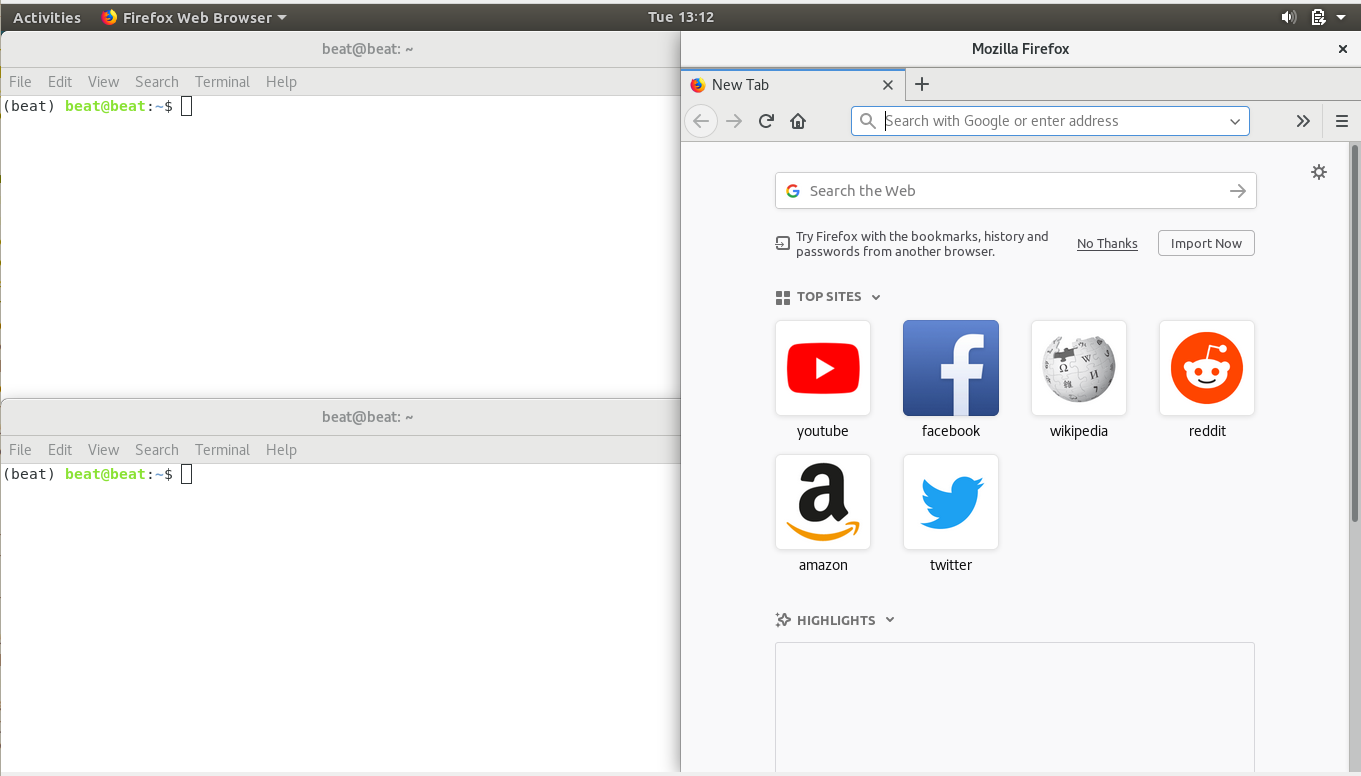
One of the terminals is for running the beat.editor server; one is for editing code and running beat.cmdline commands; the browser is for using the beat.editor web application.

A Sanity Check

Let’s make sure your installation is working as intended. Run the following in a terminal (in the parent folder of your prefix!):

$ beat exp list

This lists all the experiments in your prefix, and should not be empty.

Warning

You need your Conda environment active to access these tools & commands. If the beat command isn’t found, make sure to run conda activate <environment name>!

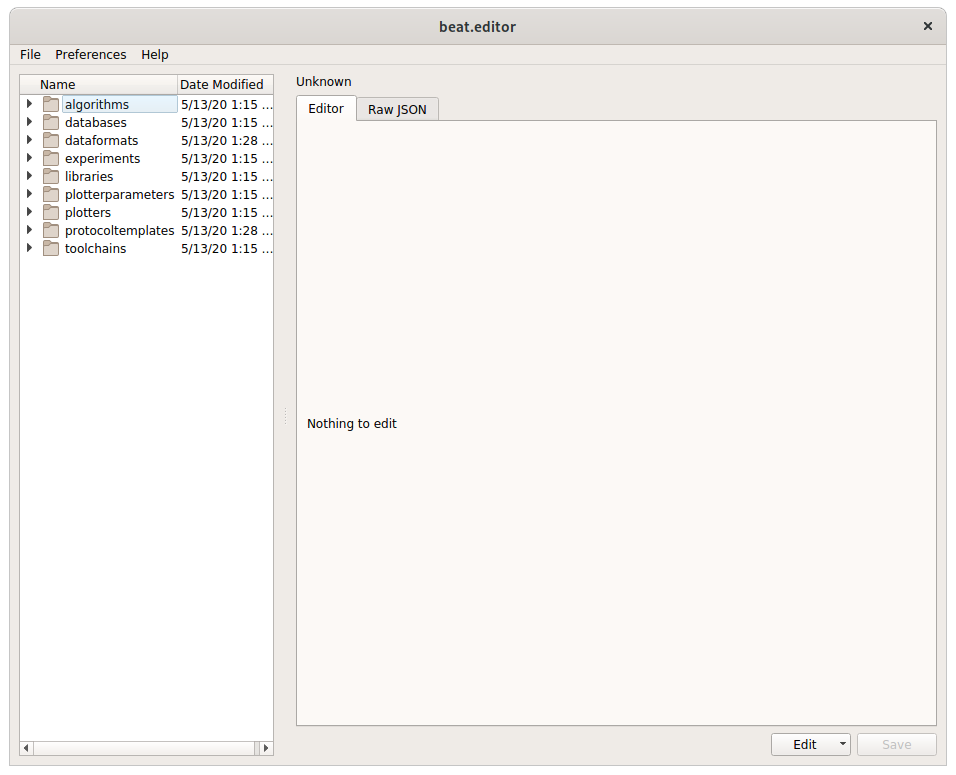
Now, let’s make sure beat.editor is working. Run the following:

$ beat editor start &

A new application should open up showing this:

The Iris LDA Experiment

This tutorial will be based on the classic Iris LDA experiment. We’ll start by explaining the problem, designing a solution, and seeing this solution in terms of BEAT. We’ll then run the experiment, analyze it, and debug it. After that we start changing parts of the experiment and creating BEAT objects to represent our changes.

The Problem: What are we doing?

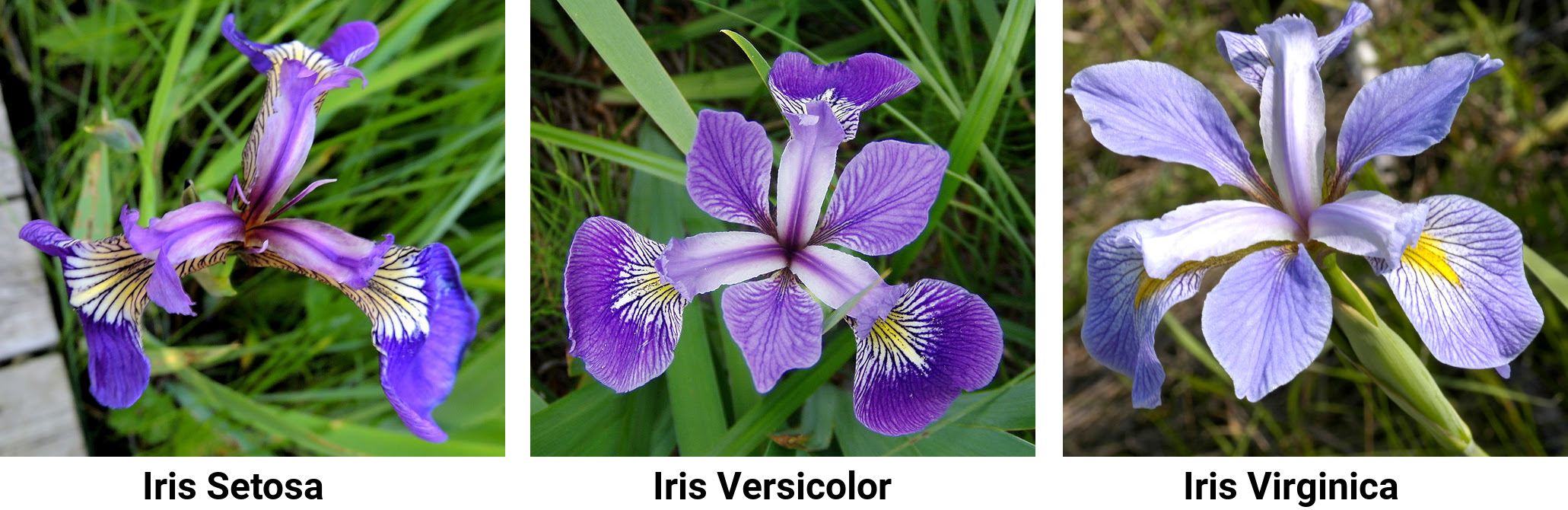
Our task will be to discriminate between the 3 types of flowers in Fisher’s Iris dataset using LDA. To keep it simple, we will just be discriminating setosa & versicolor flower samples versus virginica flower samples, giving us a 2-class problem.

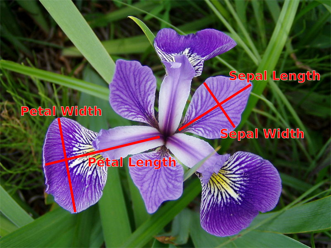
Each sample in Fisher’s Iris dataset is 4 measurements from a flower:

The dataset therefore looks like the following:

The Goal: What do we want?

We will get 3 figures of merit from running the experiment:

• The EER (Equal Error Rate).

• ROC plot.

• Scores histogram plot.

Designing our Experiment outside of BEAT

Let’s design the experiment abstractly, before showing how it is designed out of BEAT objects.

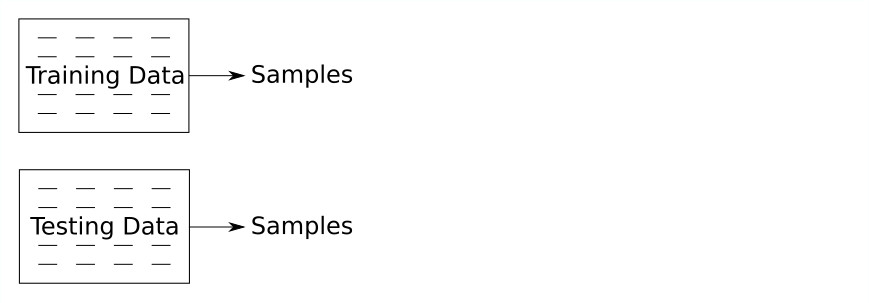
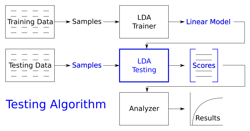
The first thing we need is the training data for training our LDA machine and the testing data to test the trained model:

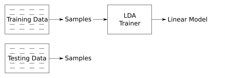
Then we need to train the LDA:

Then we test the LDA:

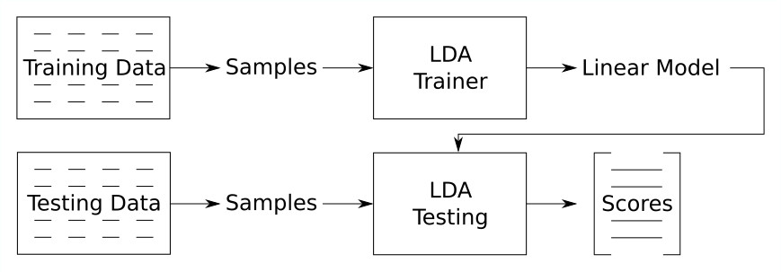
Then we analyze our scores and generate our figures of merit:

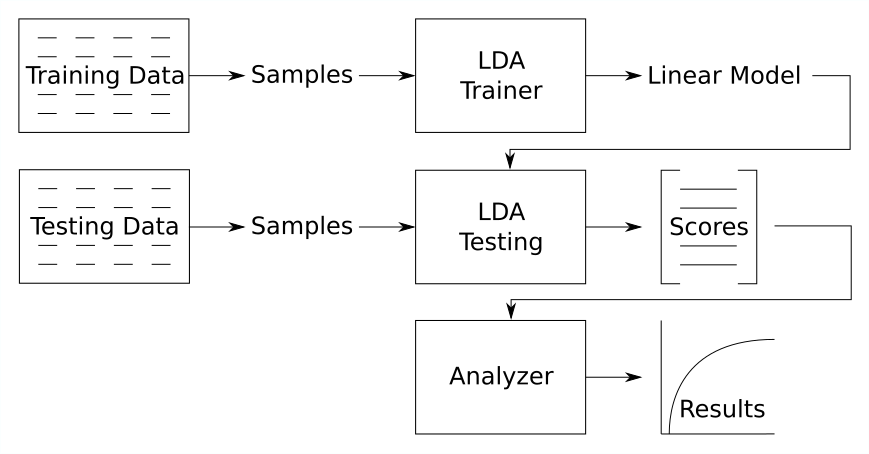
And there is our conceptual experiment diagram! You’ve probably seen and thought of designs similar to this. Let’s see how to split it into BEAT objects.

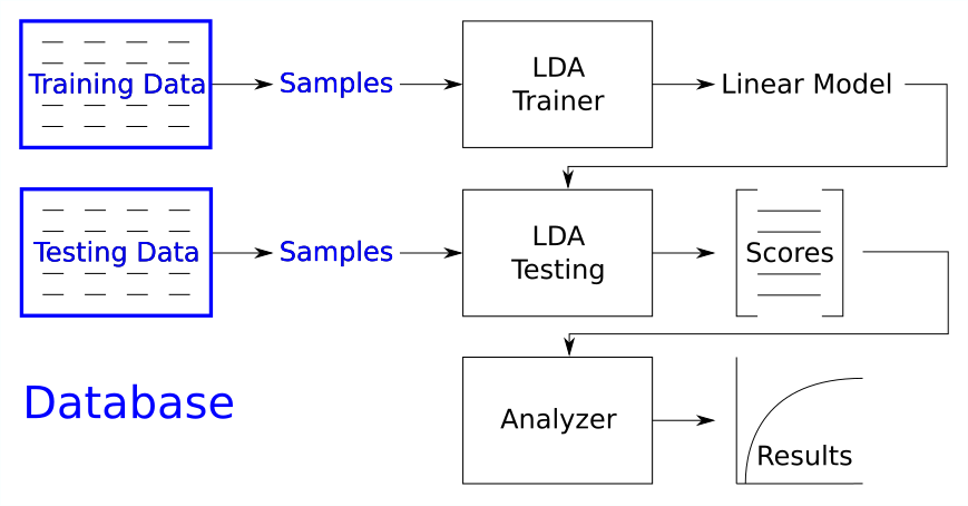
We need database block that provides data to the BEAT experiments:

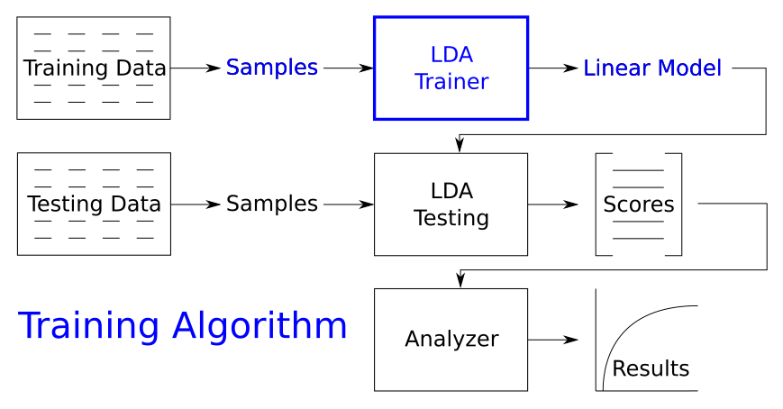
We need an algorithm for training the LDA machine:

We need another algorithm for testing the model:

And we’ll need an analyzer algorithm for generating our figures of merit:

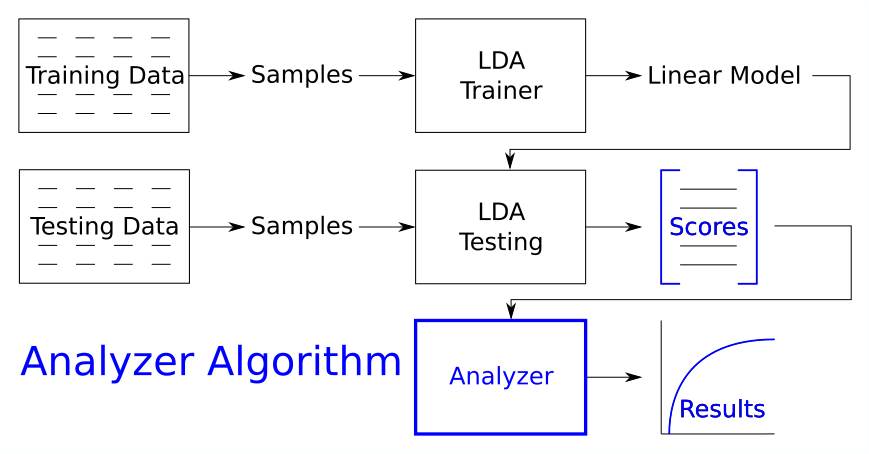
In addition to that, we will need a toolchain and an experiment. This gives us 6 different BEAT objects:

• Database

• Training algorithm

• Testing algorithm

• Analyzer algorithm

• Toolchain

• Experiment

Luckily, these are all already created for us!

Running the Iris LDA Experiment

Now that we understand what we’re doing (more or less), let’s get our hands dirty running the pre-made Iris LDA experiment. To do so, we’ll be using the BEAT command line tool from the beat.cmdline package.

Warning

Remember to run shell commands in the parent directory of your prefix!

Let’s make sure the experiment we want to run exists:

$ beat exp list

Make sure the experiment name, test/test/iris/1/iris, is in that list.

Run the experiment:

$ beat exp run test/test/iris/1/iris

It should finish successfully and output status remarks ending with a long amount of JSON-like data. Scrolling up to the top of the output, you should see the following:

Index for database iris/1 not found, building it
Index for database iris/1 not found, building it
Running `test/iris_training/1' for block `training_alg'
Start the execution of 'test/iris_training/1'
Running `test/iris_testing/1' for block `testing_alg'
Start the execution of 'test/iris_testing/1'
Running `test/iris_analyzer/1' for block `analyzer'
Start the execution of 'test/iris_analyzer/1'
  Results:
  {
    "eer": 0.019999999552965164,
    "roc": {
      "data": [
        {

See all those statements about Running `<algorithm name>` for block `<block name>`? Those are letting you know where the execution of the experiment is at. You can see that it first runs the training algorithm, test/iris_training/1, for the training_alg block. Then it runs the testing algorithm for the testing block, and finally the analyzer algorithm for the analyzer block. The results are printed last, which you can immediately print again by re-running the experiment.

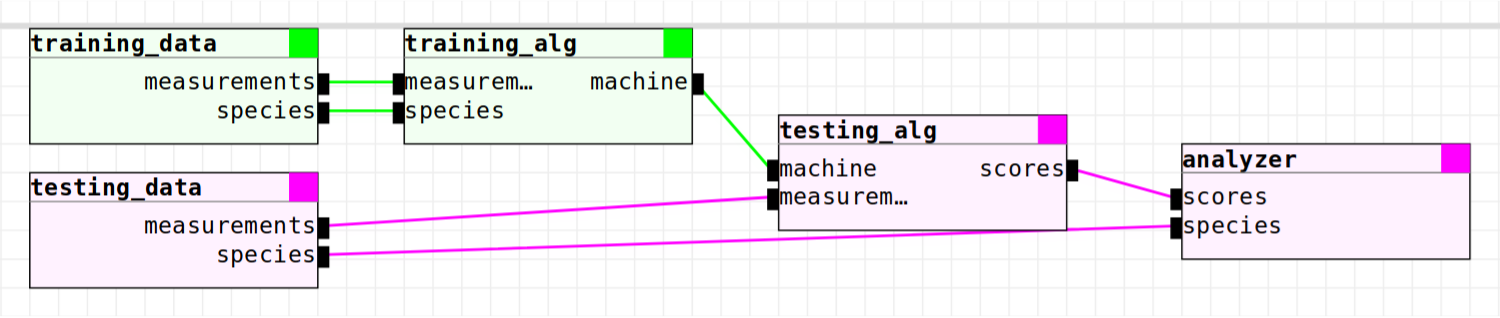
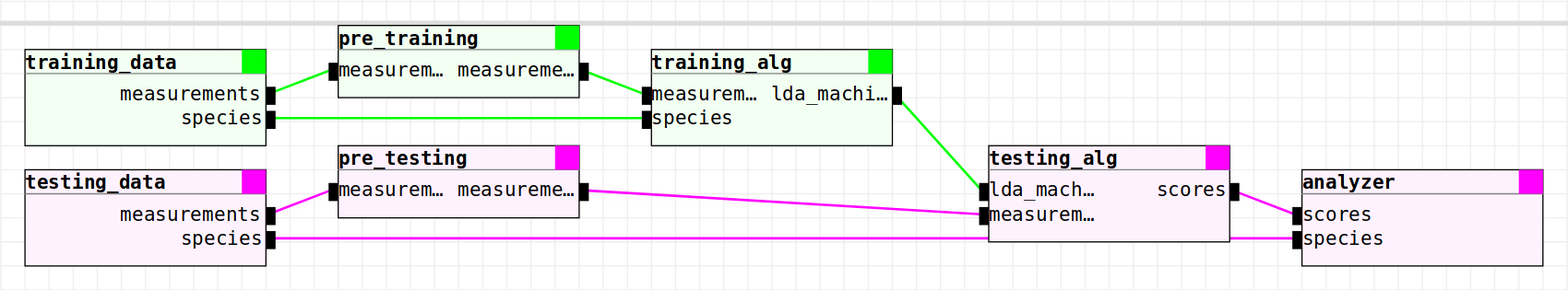
These block names are the block names from the experiment’s toolchain. Our experiment uses the test/iris/1 toolchain, which looks like this:

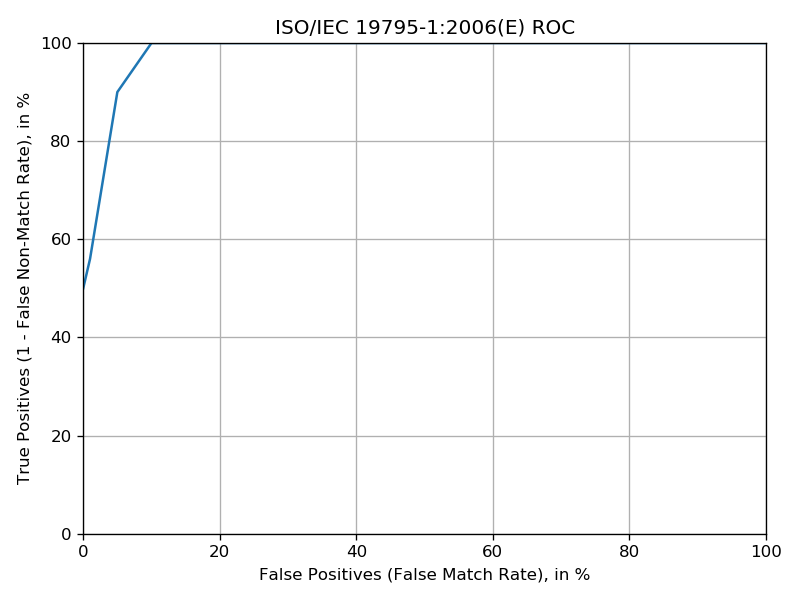
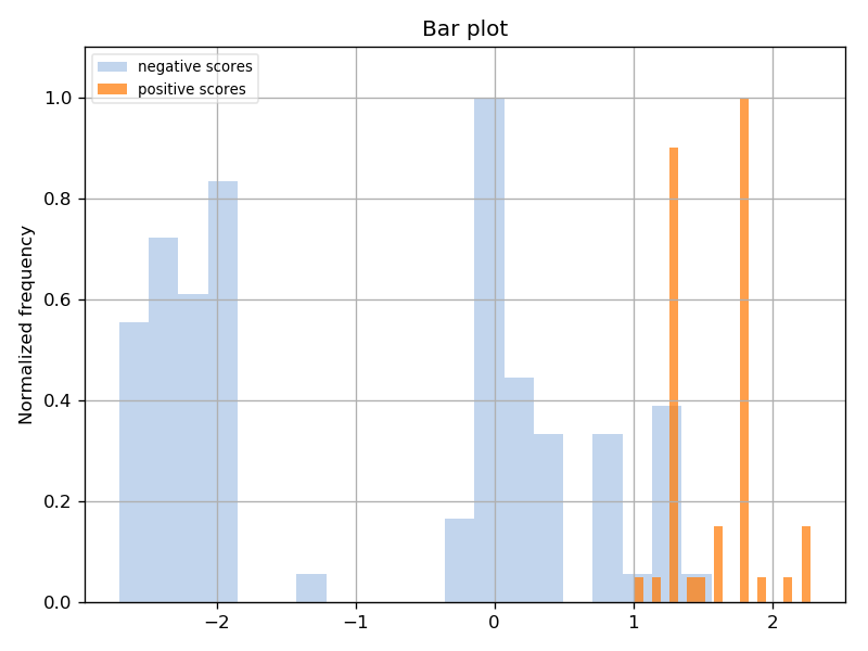
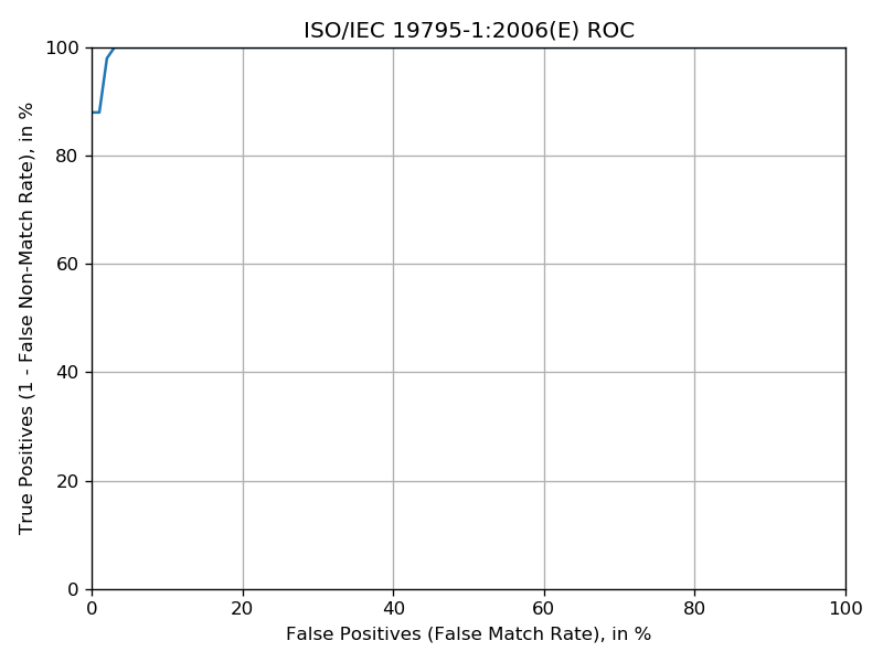
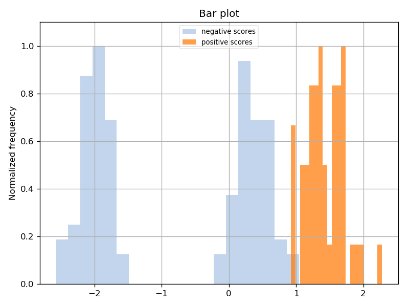
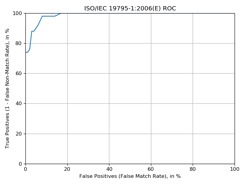
Now let’s generate the ROC and scores distribution plots! Run the following:

$ beat exp plot --show test/test/iris/1/iris

This plots our experiment’s plot table results. The --show flag tells us to pop up the plots as soon as they are generated, so we don’t have to find them in the filesystem to see them.

You should be seeing two plots, the ROC and scores distribution:

Debugging the Iris LDA Experiment

There are a couple of things to keep in mind when debugging your experiments:

1. The BEAT cache system.

2. The availability of normal Python debugging strategies.

The Cache System

There is a subfolder in your prefix called cache. This folder holds all the caches for every step of every experiment you have ran - every block, once executed, saves its results in a cache entry. The cache entry for a block is saved in a path made from hashing the metadata & code from that block and every block before it. This means the following:

• You may re-run an experiment and immediately get its results, since all of the experiment’s steps are found in the cache.

• Changing a block in an experiment (whether its a source code file or metadata) will re-run that step and every step that depends on it.

• Changing a database means that all experiments ran using that database cannot use any of their caches.

• Changing an analyzer of an experiment means that only the last step will have to be re-ran.

Note

Please note that the root folder of the database is not a part of information used for producing the hash of the database block. Therefore if the only modification in a database block is changing its root folder, BEAT will use the previous cach data available. You need to clear the cache manually to make sure that the new root folder is accessable by beat. for more information about the data used for making the hashes of each block please refer to the hash.py from beat.core.

To look at an experiment’s caches, use the beat exp caches <exp name> command. To see our experiment’s caches:

$ beat exp caches test/test/iris/1/iris

To work with caches generally:

$ beat cache

Using Debugging Strategies

Let’s run a different experiment for this: test/test/iris/1/error. This experiment purposely has a bug in its analyzer algorithm Python file:

Skipping execution of `test/iris_training/1' for block `training_alg' - outputs exist
Skipping execution of `test/iris_testing/1' for block `testing_alg' - outputs exist
Running `test/iris_analyzer_error/1' for block `analyzer'
Start the execution of 'test/iris_analyzer_error/1'
Block did not execute properly - outputs were reset
  Standard output:

  Standard error:

  Captured user error:
    File "test/iris_analyzer_error/1.py", line 55, in process
        far32 = nump.float32(far)
    NameError: name 'nump' is not defined
  Captured system error:

Let’s edit that Python file:

$ beat alg edit test/iris_analyzer_error/1

And uncomment line 53:

#print(nump)

Note

If you don’t want to edit using the beat alg edit command (e.g., an external editor), you can find the path of the file to edit by using beat alg path instead of beat alg edit and copying the file path.

Save the file, exit the editor, and re-run the experiment again, to get the following message:

...
  Captured user error:
    File "test/iris_analyzer_error/1.py", line 53, in process
        print(nump)
    NameError: name 'nump' is not defined
  Captured system error:

Now we know for sure that “nump” isn’t defined. To make very sure, let’s inspect it with ipdb. Edit the file again with:

$ beat alg edit test/iris_analyzer_error/1

Recomment line 53 and uncomment line 54:

#import ipdb;ipdb.set_trace()

Run the experiment again to be put into an ipdb prompt when the block executes! You can play around in here like normal, and make sure that “nump” was just a misspelling of “numpy”.

The Iris Means Experiment

Let’s start learning how to use beat.editor! We will start off by copying our experiment test/test/iris/1/iris and changing the LDA algorithm to a more simple means-based algorithm:

1. In the training step, we will calculate the mean measurement of setosa and versicolor flower samples (averaging all our “negative samples”).

2. In the testing step, we will compare all our samples to this mean sample by calculating the distance from the current sample to the mean sample.

Warning

Make sure the beat editor serve server is running in a terminal tab in the parent directory of your prefix!

Creating the Experiment

In the BEAT editor browser tab, click the “experiments” tab on the top navigation bar. This will show you a list of experiments, including the Iris LDA experiment test/test/iris/1/iris.

Click the Clone button next to the Iris LDA experiment. This will pop up a window for creating your new experiment, with the “User”, “Toolchain”, and “Name” fields already pre-filled with the values from the cloned Iris LDA experiment. Note that it says “Invalid Name” at the top, because the name is already taken.

Change the “User” field from “test” to “tutorial” (or your own name), and change the “Name” field from “iris” to “means”. Click the Create button to create your new experiment! You should see your new Iris Means experiment at the top of the experiment list.

Click on your Iris Means experiment’s name to go into the Experiment Editor for that experiment. We are going to change this copied experiment from using LDA as its algorithm to using our means algorithm. These two algorithms are already created - test/means_training/1 and test/means_testing/1.

Note

Please see the Experiment Editor documentation section for information on what constitutes the editor.

In the toolchain window, click on the training_alg block to open the block editor for that block. Under the toolchain window, change the selected algorithm for the training_alg block under the “Algorithm” select box from test/iris_training/1 to test/means_training/1.

In the toolchain window, click on the testing_alg block to open the block editor for that block. Under the toolchain window, change the selected algorithm for the testing_alg block under the “Algorithm” select box from test/iris_testing/1 to test/means_testing/1.

Click the Save Changes button at the top to save your changes to your Iris Means experiment. We have finished our editing - now to run it!

Running & Analyzing the Experiment

Back in your terminal, check to make sure the new experiment is in your prefix:

$ beat exp list

You should see your experiment (tutorial/test/iris/1/means). Now run it like we did earlier:

$ beat exp run tutorial/test/iris/1/means

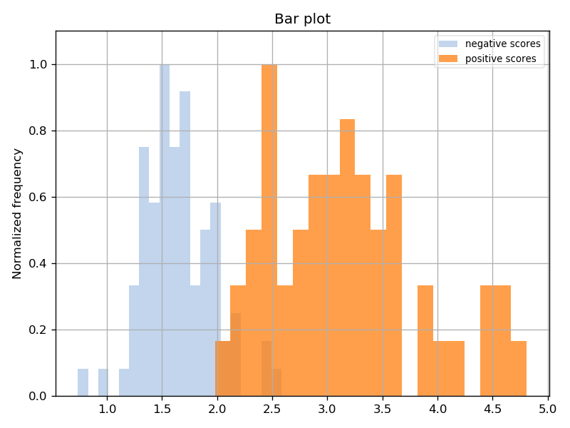
You should see output similar to the output you saw for the Iris LDA experiment. Let’s plot the ROC and scores distribution:

$ beat exp plot --show test/test/iris/1/iris

You should see the following two plots:

The Advanced Iris Experiment

Many experiments will use a preprocessing step. Right now, our Iris experiments don’t have one. Let’s add one!

Our preprocessing algorithm will be very simple (and not particularly useful) - round each measurement in a sample to the nearest whole number.

The dataset, currently:

The dataset, after being preprocessed:

Everything else will be the same as the Iris LDA experiment.

Changing the Toolchain

The first thing we need to do is make a toolchain for this experiment with blocks for the preprocessor. We copy our Iris toolchain, test/iris/1:

And edit our copy to look like:

Go to your beat.editor browser tab. Click on the toolchains button at the top to go to your toolchains list. You should see the test/iris/1 toolchain and a couple others.

Do the same we did for the experiment: click the Clone button and change the “User” & “Name” fields from “test” and “iris” to “tutorial” and “iris_advanced”, respectively. Click Create to save the toolchain, and click on the new toolchain’s name to open up the Toolchain Editor for this object.

Note

Please see the Toolchain Editor documentation section for information on what constitutes the editor.

Now we will add the preprocessor blocks to the toolchain. Do the following steps:

1. Scroll down to fit the toolchain window editor in your browser window. Make sure that you can see the toolchain blocks. If you can’t, click on the Fit button in the top-right menu in the editor to fit the blocks to your screen.

2. We need to make space for the new blocks: Shift over the last three blocks (training_alg, testing_alg, and analyzer) to make space for the preprocessor blocks. Left-click and drag to area-select all three of these blocks. Left-click and drag on the grey rectangle encompassing these three blocks to the right to move your selection to the right. Click anywhere outside of the grey rectangle to deselect the blocks.

3. We need to remove the connections that need the preprocessing step: Right click on the connection going from training_data’s “measurements” output to training_alg’s “measurements” input. Select Delete Connection to remove the connection. Do the same for the other “measurements” connection for the testing data.

4. We need to create the preprocessor blocks: Right-click between the training_data and training_alg blocks to open the block insertion menu. Click Create Block Here to insert a new block at your cursor. Add another block between the testing_data and testing_alg blocks.

5. We need to edit the new blocks to change their names and add inputs & outputs: Click on the new block between the “training” blocks to open the Block Editor modal. Change the name from “block” to “pre_training”. Click Add Input and Add Output - rename both of these to “measurements”. Click the “X” button in the top right, press the “Esc” button on your keyboard, or click out of the modal to close the editor. Do the same for the other new block, but name it “pre_testing”.

6. Now that we have our preprocessor blocks, we need to connect the blocks to the rest of the toolchain: Click and drag on the black square next to the “measurements” output of the training_data block to start creating a connection. Drag and release this connection on the black square next to pre_training’s “measurements” input. Create another connection from pre_training’s “measurements” output to training_alg’s “measurements” input. Do the same for the test data preprocessor block.

7. Make sure the synchronization channels are properly set: The pre_training block should be green (synchronized to the training_data channel), and the pre_testing block should be pink (synchronized to the testing_data channel). If not, click on the blocks and change the “Channel” to the appropriate channel.

8. You should have the same toolchain as shown above! Now we can create our preprocessor algorithm and use it in a experiment.

Creating the Preprocessor Algorithm

We need an algorithm to fill in our preprocessors blocks in our toolchain. Let’s create a new algorithm.

Click on algorithms at the top of your beat.editor browser tab to go to the list of your algorithms in your prefix. You should see the algorithms you’ve been using as well as others.

Click the New button in the top right of the list to pop up the modal for creating objects. Fill in the “User” and “Name” fields with “tutorial” and “iris_preprocessor”.

Click Create to create the new algorithm, tutorial/iris_preprocessor/1, at the top of your algorithms list. Click on the new algorithm’s name to enter the Algorithm Editor for this algorithm.

Note

Please see the Algorithm Editor documentation section for information on what constitutes the editor.

Our preprocessor algorithm takes in a sample (set of 4 measurements), rounds the measurements, and returns the rounded sample. This means that the algorithm will have 1 group with 1 input and 1 output. Do the following steps:

1. Click the New Group button at the bottom of the page to add a new group, if one doesn’t already exist.

2. Click the New Input and New Output buttons if the group doesn’t already have any.

3. Rename the input and the output to “measurements”.

4. The algorithm metadata is complete! Click Save Changes at the top to save the new algorithm. Click the Generate Python File to generate a basic python file for this algorithm based off a template.

5. Back in the shell, run the following to start editing this python file:

   $ beat alg edit tutorial/iris_advanced/1
   

6. Add the following code to the end of the process method, before the return statement:

   # get the array of measurements
   measurements = inputs['measurements'].data.value
   # round each measurement
   processed = [round(m) for m in measurements]
   # output the new array
   outputs['measurements'].write({
     'value': processed
   })
   

7. Save and exit your editor. Now the algorithm is done! Time to create the experiment and see how useful this preprocessor is.

Creating the Iris Advanced Experiment

Click the experiments tab to go to your experiments list. Click New to create a new experiment:

1. Fill in the “Name” field with “tutorial”

2. Select your new toolchain (tutorial/iris_advanced/1) in the “Toolchain” field

3. Fill in the “Name” field with “iris”

4. Click Create to create the experiment

Click the new experiment’s name to enter the Experiment Editor for this experiment.

Before, we just changed an experiment. Now, we have to fill in an entire experiment from scratch. This means that we have to assign the correct dataset & algorithm for each block in the toolchain.

Refer to the Iris LDA experiment for the correct datasets & algorithms for all blocks except the preprocessor blocks, pre_training and pre_testing. For these two, choose the algorithm we just created, tutorial/iris_preprocessor/1.

Now save the experiment, and run it! Back in the terminal, check to make sure the experiment exists:

$ beat exp list

Run the experiment:

$ beat exp run tutorial/tutorial/iris_advanced/1/iris

Plot the experiment:

$ beat exp plot --show tutorial/tutorial/iris_advanced/1/iris

You should see the following two diagrams: