User guide
The EM algorithm is an iterative method that estimates parameters for statistical models, where the model depends on unobserved latent variables. The EM iteration alternates between performing an expectation (E) step, which creates a function for the expectation of the log-likelihood evaluated using the current estimate for the parameters, and a maximization (M) step, which computes parameters maximizing the expected log-likelihood found on the E step. These parameter-estimates are then used to determine the distribution of the latent variables in the next E step 8.
Machines and trainers are the core components of Bob’s machine learning packages. Machines represent statistical models or other functions defined by parameters that can be learned by trainers or manually set. Below you will find machine/trainer guides for learning techniques available in this package.
K-Means
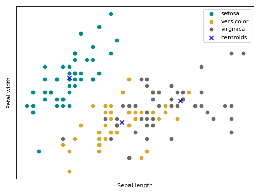
k-means 7 is a clustering method which aims to partition a set of \(N\) observations into \(C\) clusters with equal variance minimizing the following cost function \(J = \sum_{i=0}^{N} \min_{\mu_j \in C} ||x_i - \mu_j||\), where \(\mu\) is a given mean (also called centroid) and \(x_i\) is an observation.
This implementation has two stopping criteria. The first one is when the maximum number of iterations is reached; the second one is when the difference between \(Js\) of successive iterations are lower than a convergence threshold.
In this implementation, the training consists in the definition of the
statistical model, called machine, (bob.learn.em.KMeansMachine) and
this statistical model is learned by executing the
fit() method.
Follow bellow an snippet on how to train a KMeans using Bob.
>>> from bob.learn.em import KMeansMachine
>>> import numpy
>>> data = numpy.array(
...     [[3,-3,100],
...      [4,-4,98],
...      [3.5,-3.5,99],
...      [-7,7,-100],
...      [-5,5,-101]], dtype='float64')
>>> # Create a k-means machine with k=2 clusters
>>> kmeans_machine = KMeansMachine(2, convergence_threshold=1e-5, max_iter=200)
>>> # Train the KMeansMachine
>>> kmeans_machine = kmeans_machine.fit(data)
>>> print(numpy.array(kmeans_machine.centroids_))
[[   3.5   -3.5   99. ]
 [  -6.     6.  -100.5]]
Bellow follow an intuition (source code + plot) of a kmeans training using the Iris flower dataset.
(Source code, png, hires.png, pdf)

Gaussian mixture models
A Gaussian mixture model (GMM) is a probabilistic model for density estimation. It assumes that all the data points are generated from a mixture of a finite number of Gaussian distributions. More formally, a GMM can be defined as: \(P(x|\Theta) = \sum_{c=0}^{C} \omega_c \mathcal{N}(x | \mu_c, \sigma_c)\) , where \(\Theta = \{ \omega_c, \mu_c, \sigma_c \}\).
This statistical model is defined in the class
bob.learn.em.GMMMachine as bellow.
>>> import bob.learn.em
>>> # Create a GMM with k=2 Gaussians
>>> gmm_machine = bob.learn.em.GMMMachine(n_gaussians=2)
There are plenty of ways to estimate \(\Theta\); the next subsections explains some that are implemented in Bob.
Maximum likelihood Estimator (MLE)
In statistics, maximum likelihood estimation (MLE) is a method of estimating
the parameters of a statistical model given observations by finding the
\(\Theta\) that maximizes \(P(x|\Theta)\) for all \(x\) in your
dataset 9. This optimization is done by the Expectation-Maximization
(EM) algorithm 8 and it is implemented by
bob.learn.em.GMMMachine by setting the keyword argument trainer=”ml”.
A very nice explanation of EM algorithm for the maximum likelihood estimation can be found in this Mathematical Monk YouTube video.
Follow bellow an snippet on how to train a GMM using the maximum likelihood estimator.
>>> import bob.learn.em
>>> import numpy
>>> data = numpy.array(
...     [[3,-3,100],
...      [4,-4,98],
...      [3.5,-3.5,99],
...      [-7,7,-100],
...      [-5,5,-101]], dtype='float64')
>>> # Create a kmeans model (machine) m with k=2 clusters
>>> # and using the MLE trainer to train the GMM:
>>> # In this setup, kmeans is used to initialize the means, variances and weights of the gaussians
>>> gmm_machine = bob.learn.em.GMMMachine(n_gaussians=2, trainer="ml")
>>> # Training
>>> gmm_machine = gmm_machine.fit(data)
>>> print(gmm_machine.means)
 [[   3.5   -3.5   99. ]
  [  -6.     6.  -100.5]]
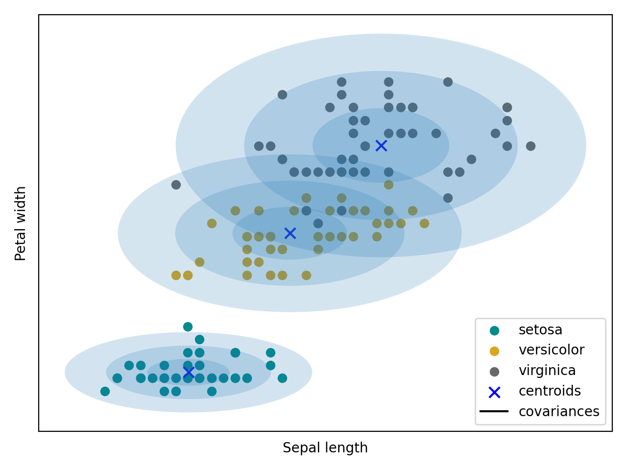
Bellow follow an intuition of the GMM trained the maximum likelihood estimator using the Iris flower dataset.
(Source code, png, hires.png, pdf)

Maximum a posteriori Estimator (MAP)
Closely related to the MLE, Maximum a posteriori probability (MAP) is an
estimate that equals the mode of the posterior distribution by incorporating in
its loss function a prior distribution 10. Commonly this prior distribution
(the values of \(\Theta\)) is estimated with MLE. This optimization is done
by the Expectation-Maximization (EM) algorithm 8 and it is implemented
by bob.learn.em.GMMMachine by setting the keyword argument trainer=”map”.
A compact way to write relevance MAP adaptation is by using GMM supervector notation (this will be useful in the next subsections). The GMM supervector notation consists of taking the parameters of \(\Theta\) (weights, means and covariance matrices) of a GMM and create a single vector or matrix to represent each of them. For each Gaussian component \(c\), we can represent the MAP adaptation as the following \(\mu_i = m + d_i\), where \(m\) is our prior and \(d_i\) is the class offset.
Follow bellow an snippet on how to train a GMM using the MAP estimator.
>>> import bob.learn.em
>>> import numpy
>>> data = numpy.array(
...     [[3,-3,100],
...      [4,-4,98],
...      [3.5,-3.5,99],
...      [-7,7,-100],
...      [-5,5,-101]], dtype='float64')
>>> # Creating a fake prior
>>> prior_gmm = bob.learn.em.GMMMachine(2)
>>> # Set some random means/variances and weights for the example
>>> prior_gmm.means = numpy.array(
...     [[ -4.,   2.3,  -10.5],
...      [  2.5, -4.5,   59. ]])
>>> prior_gmm.variances = numpy.array(
...     [[ -0.1,   0.5,  -0.5],
...      [  0.5, -0.5,   0.2 ]])
>>> prior_gmm.weights = numpy.array([ 0.8,   0.5])
>>> # Creating the model for the adapted GMM, and setting the `prior_gmm` as the source GMM
>>> # note that we have set `trainer="map"`, so we use the Maximum a posteriori estimator
>>> adapted_gmm = bob.learn.em.GMMMachine(2, ubm=prior_gmm, trainer="map")
>>> # Training
>>> adapted_gmm = adapted_gmm.fit(data)
>>> print(adapted_gmm.means)
 [[ -4.      2.3   -10.5  ]
  [  0.944  -1.833  36.889]]
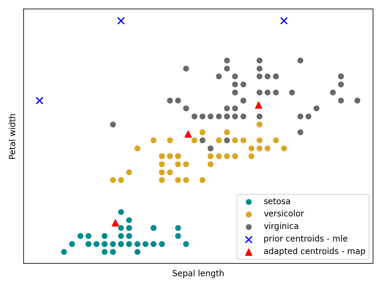
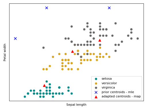
Bellow follow an intuition of the GMM trained with the MAP estimator using the Iris flower dataset. It can be observed how the MAP means (the red triangles) around the center of each class from a prior GMM (the blue crosses).
(Source code, png, hires.png, pdf)
Session Variability Modeling with Gaussian Mixture Models
In the aforementioned GMM based algorithms there is no explicit modeling of session variability. This section will introduce some session variability algorithms built on top of GMMs.
GMM statistics
Before introduce session variability for GMM based algorithms, we must
introduce a component called bob.learn.em.GMMStats. This component
is useful for some computation in the next sections.
bob.learn.em.GMMStats is a container that solves the Equations 8, 9
and 10 in [Reynolds2000] (also called, zeroth, first and second order GMM
statistics).
Given a GMM (\(\Theta\)) and a set of samples \(x_t\) this component accumulates statistics for each Gaussian component \(c\).
Follow bellow a 1-1 relationship between statistics in [Reynolds2000] and the
properties in bob.learn.em.GMMStats:
Eq (8) is
bob.learn.em.GMMStats.n: \(n_c=\sum\limits_{t=1}^T Pr(c | x_t)\) (also called responsibilities)Eq (9) is
bob.learn.em.GMMStats.sum_px: \(E_c(x)=\frac{1}{n(c)}\sum\limits_{t=1}^T Pr(c | x_t)x_t\)Eq (10) is
bob.learn.em.GMMStats.sum_pxx: \(E_c(x^2)=\frac{1}{n(c)}\sum\limits_{t=1}^T Pr(c | x_t)x_t^2\)
where \(T\) is the number of samples used to generate the stats.
The snippet bellow shows how to compute accumulated these statistics given a prior GMM.
 >>> import bob.learn.em
 >>> import numpy
 >>> numpy.random.seed(10)
 >>>
 >>> data = numpy.array(
 ...     [[0, 0.3, -0.2],
 ...      [0.4, 0.1, 0.15],
 ...      [-0.3, -0.1, 0],
 ...      [1.2, 1.4, 1],
 ...      [0.8, 1., 1]], dtype='float64')
 >>> # Training a GMM with 2 Gaussians of dimension 3
 >>> prior_gmm = bob.learn.em.GMMMachine(2).fit(data)
 >>> # Creating the container
 >>> gmm_stats = prior_gmm.acc_stats(data)
 >>> # Printing the responsibilities
 >>> print(gmm_stats.n/gmm_stats.t)
  [0.6  0.4]
Inter-Session Variability
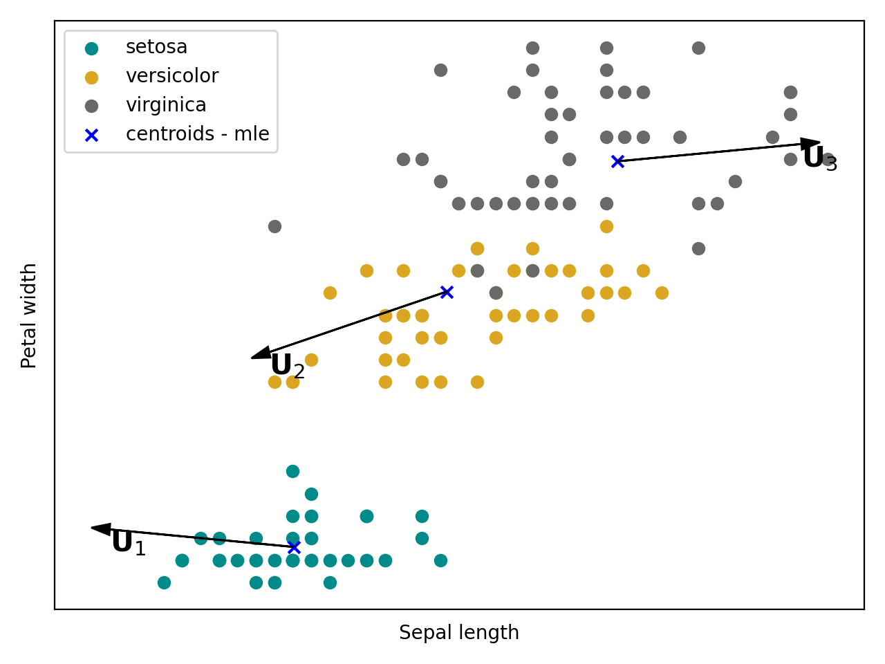
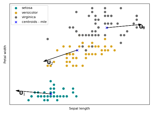
Inter-Session Variability (ISV) modeling 3 2 is a session variability modeling technique built on top of the Gaussian mixture modeling approach. It hypothesizes that within-class variations are embedded in a linear subspace in the GMM means subspace, and these variations can be suppressed by an offset w.r.t each mean during the MAP adaptation.
In this generative model, each sample is assumed to have been generated by a GMM mean supervector with the following shape: \(\mu_{i, j} = m + Ux_{i, j} + D_z{i}\), where \(m\) is our prior, \(Ux_{i, j}\) is the session offset that we want to suppress and \(D_z{i}\) is the class offset (with all session effects suppressed).
It is hypothesized that all possible sources of session variations are embedded in this matrix \(U\). Follow below an intuition of what is modeled with \(U\) in the Iris flower dataset. The arrows \(U_{1}\), \(U_{2}\) and \(U_{3}\) are the directions of the within-class variations, with respect to each Gaussian component, that will be suppressed a posteriori.
(Source code, png, hires.png, pdf)
The ISV statistical model is stored in this container
bob.learn.em.ISVMachine.
The snippet bellow shows how to:
Train a Intersession variability modeling.
Enroll a subject with such a model.
Compute score with such a model.
>>> import bob.learn.em
>>> import numpy as np

>>> np.random.seed(10)

>>> # Generating some fake data
>>> data_class1 = np.random.normal(0, 0.5, (10, 3))
>>> data_class2 = np.random.normal(-0.2, 0.2, (10, 3))
>>> X = np.vstack((data_class1, data_class2))
>>> y = np.hstack((np.zeros(10, dtype=int), np.ones(10, dtype=int)))
>>> # Create an ISV machine with a UBM of 2 gaussians
>>> isv_machine = bob.learn.em.ISVMachine(r_U=2, ubm_kwargs=dict(n_gaussians=2))
>>> _ = isv_machine.fit_using_array(X, y)  # DOCTEST: +SKIP_
>>> # Alternatively, you can create a pipeline of a GMMMachine and an ISVMachine
>>> # and call pipeline.fit(X, y) instead of calling isv.fit_using_array(X, y)
>>> isv_machine.U
  array(...)

>>> # Enrolling a subject
>>> enroll_data = np.array([[1.2, 0.1, 1.4], [0.5, 0.2, 0.3]])
>>> model = isv_machine.enroll_using_array(enroll_data)
>>> print(model)
  [[ 0.54   0.246  0.505  1.617 -0.791  0.746]]

>>> # Probing
>>> probe_data = np.array([[1.2, 0.1, 1.4], [0.5, 0.2, 0.3]])
>>> score = isv_machine.score_using_array(model, probe_data)
>>> print(score)
  [2.754]
Joint Factor Analysis
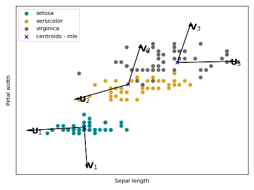
Joint Factor Analysis (JFA) 1 2 is an extension of ISV. Besides the within-class assumption (modeled with \(U\)), it also hypothesize that between class variations are embedded in a low rank rectangular matrix \(V\). In the supervector notation, this modeling has the following shape: \(\mu_{i, j} = m + Ux_{i, j} + Vy_{i} + D_z{i}\).
Follow bellow an intuition of what is modeled with \(U\) and \(V\) in the Iris flower dataset. The arrows \(V_{1}\), \(V_{2}\) and \(V_{3}\) are the directions of the between class variations with respect to each Gaussian component that will be added a posteriori.
(Source code, png, hires.png, pdf)

The JFA statistical model is stored in this container
bob.learn.em.JFAMachine. The snippet bellow shows how to train a
such session variability model.
Train a JFA model.
Enroll a subject with such a model.
Compute score with such a model.
>>> import bob.learn.em
>>> import numpy as np

>>> np.random.seed(10)

>>> # Generating some fake data
>>> data_class1 = np.random.normal(0, 0.5, (10, 3))
>>> data_class2 = np.random.normal(-0.2, 0.2, (10, 3))
>>> X = np.vstack((data_class1, data_class2))
>>> y = np.hstack((np.zeros(10, dtype=int), np.ones(10, dtype=int)))
>>> # Create a JFA machine with a UBM of 2 gaussians
>>> jfa_machine = bob.learn.em.JFAMachine(r_U=2, r_V=2, ubm_kwargs=dict(n_gaussians=2))
>>> _ = jfa_machine.fit_using_array(X, y)
>>> jfa_machine.U
  array(...)

>>> enroll_data = np.array([[1.2, 0.1, 1.4], [0.5, 0.2, 0.3]])
>>> model = jfa_machine.enroll_using_array(enroll_data)
>>> print(model)
  (array([0.634, 0.165]), array([ 0.,  0.,  0.,  0., -0.,  0.]))

>>> probe_data = np.array([[1.2, 0.1, 1.4], [0.5, 0.2, 0.3]])
>>> score = jfa_machine.score_using_array(model, probe_data)
>>> print(score)
  [0.471]