User guide
The EM algorithm is an iterative method that estimates parameters for statistical models, where the model depends on unobserved latent variables. The EM iteration alternates between performing an expectation (E) step, which creates a function for the expectation of the log-likelihood evaluated using the current estimate for the parameters, and a maximization (M) step, which computes parameters maximizing the expected log-likelihood found on the E step. These parameter-estimates are then used to determine the distribution of the latent variables in the next E step [8].
Machines and trainers are the core components of Bob’s machine learning packages. Machines represent statistical models or other functions defined by parameters that can be learned by trainers or manually set. Below you will find machine/trainer guides for learning techniques available in this package.
K-Means
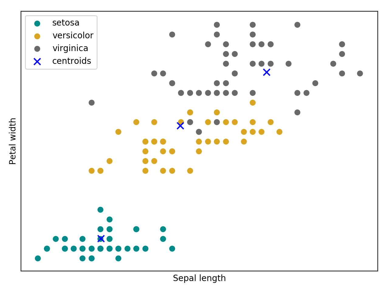
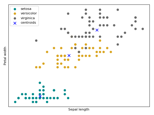
k-means [7] is a clustering method which aims to partition a set of \(N\) observations into \(C\) clusters with equal variance minimizing the following cost function \(J = \sum_{i=0}^{N} \min_{\mu_j \in C} ||x_i - \mu_j||\), where \(\mu\) is a given mean (also called centroid) and \(x_i\) is an observation.
This implementation has two stopping criteria. The first one is when the maximum number of iterations is reached; the second one is when the difference between \(Js\) of successive iterations are lower than a convergence threshold.
In this implementation, the training consists in the definition of the
statistical model, called machine, (bob.learn.em.KMeansMachine) and
this statistical model is learned via a trainer
(bob.learn.em.KMeansTrainer).
Follow bellow an snippet on how to train a KMeans using Bob.
>>> import bob.learn.em
>>> import numpy
>>> data = numpy.array(
...     [[3,-3,100],
...      [4,-4,98],
...      [3.5,-3.5,99],
...      [-7,7,-100],
...      [-5,5,-101]], dtype='float64')
>>> # Create a kmeans m with k=2 clusters with a dimensionality equal to 3
>>> kmeans_machine = bob.learn.em.KMeansMachine(2, 3)
>>> kmeans_trainer = bob.learn.em.KMeansTrainer()
>>> max_iterations = 200
>>> convergence_threshold = 1e-5
>>> # Train the KMeansMachine
>>> bob.learn.em.train(kmeans_trainer, kmeans_machine, data,
...     max_iterations=max_iterations,
...     convergence_threshold=convergence_threshold)
>>> print(kmeans_machine.means)
[[ -6.   6.  -100.5]
 [  3.5 -3.5   99. ]]
Bellow follow an intuition (source code + plot) of a kmeans training using the Iris flower dataset.
(Source code, png, hires.png, pdf)

Gaussian mixture models
A Gaussian mixture model (GMM) is a probabilistic model for density estimation. It assumes that all the data points are generated from a mixture of a finite number of Gaussian distributions. More formally, a GMM can be defined as: \(P(x|\Theta) = \sum_{c=0}^{C} \omega_c \mathcal{N}(x | \mu_c, \sigma_c)\) , where \(\Theta = \{ \omega_c, \mu_c, \sigma_c \}\).
This statistical model is defined in the class
bob.learn.em.GMMMachine as bellow.
>>> import bob.learn.em
>>> # Create a GMM with k=2 Gaussians with the dimensionality of 3
>>> gmm_machine = bob.learn.em.GMMMachine(2, 3)
There are plenty of ways to estimate \(\Theta\); the next subsections explains some that are implemented in Bob.
Maximum likelihood Estimator (MLE)
In statistics, maximum likelihood estimation (MLE) is a method of estimating
the parameters of a statistical model given observations by finding the
\(\Theta\) that maximizes \(P(x|\Theta)\) for all \(x\) in your
dataset [9]. This optimization is done by the Expectation-Maximization
(EM) algorithm [8] and it is implemented by
bob.learn.em.ML_GMMTrainer.
A very nice explanation of EM algorithm for the maximum likelihood estimation can be found in this Mathematical Monk YouTube video.
Follow bellow an snippet on how to train a GMM using the maximum likelihood estimator.
>>> import bob.learn.em
>>> import numpy
>>> data = numpy.array(
...     [[3,-3,100],
...      [4,-4,98],
...      [3.5,-3.5,99],
...      [-7,7,-100],
...      [-5,5,-101]], dtype='float64')
>>> # Create a kmeans model (machine) m with k=2 clusters
>>> # with a dimensionality equal to 3
>>> gmm_machine = bob.learn.em.GMMMachine(2, 3)
>>> # Using the MLE trainer to train the GMM:
>>> # True, True, True means update means/variances/weights at each
>>> # iteration
>>> gmm_trainer = bob.learn.em.ML_GMMTrainer(True, True, True)
>>> # Setting some means to start the training.
>>> # In practice, the output of kmeans is a good start for the MLE training
>>> gmm_machine.means = numpy.array(
...     [[ -4.,   2.3,  -10.5],
...      [  2.5, -4.5,   59. ]])
>>> max_iterations = 200
>>> convergence_threshold = 1e-5
>>> # Training
>>> bob.learn.em.train(gmm_trainer, gmm_machine, data,
...                    max_iterations=max_iterations,
...                    convergence_threshold=convergence_threshold)
>>> print(gmm_machine.means)
[[ -6.   6.  -100.5]
 [  3.5 -3.5   99. ]]
Bellow follow an intuition of the GMM trained the maximum likelihood estimator using the Iris flower dataset.
(Source code, png, hires.png, pdf)
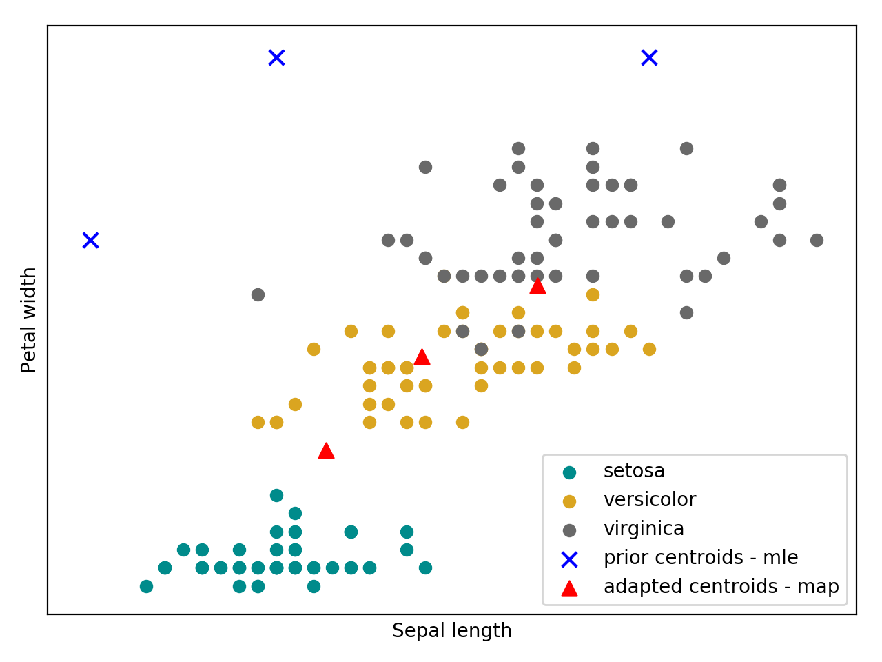
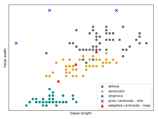
Maximum a posteriori Estimator (MAP)
Closely related to the MLE, Maximum a posteriori probability (MAP) is an
estimate that equals the mode of the posterior distribution by incorporating in
its loss function a prior distribution [10]. Commonly this prior distribution
(the values of \(\Theta\)) is estimated with MLE. This optimization is done
by the Expectation-Maximization (EM) algorithm [8] and it is implemented
by bob.learn.em.MAP_GMMTrainer.
A compact way to write relevance MAP adaptation is by using GMM supervector notation (this will be useful in the next subsections). The GMM supervector notation consists of taking the parameters of \(\Theta\) (weights, means and covariance matrices) of a GMM and create a single vector or matrix to represent each of them. For each Gaussian component \(c\), we can represent the MAP adaptation as the following \(\mu_i = m + d_i\), where \(m\) is our prior and \(d_i\) is the class offset.
Follow bellow an snippet on how to train a GMM using the MAP estimator.
>>> import bob.learn.em
>>> import numpy
>>> data = numpy.array(
...     [[3,-3,100],
...      [4,-4,98],
...      [3.5,-3.5,99],
...      [-7,7,-100],
...      [-5,5,-101]], dtype='float64')
>>> # Creating a fake prior
>>> prior_gmm = bob.learn.em.GMMMachine(2, 3)
>>> # Set some random means for the example
>>> prior_gmm.means = numpy.array(
...     [[ -4.,   2.3,  -10.5],
...      [  2.5, -4.5,   59. ]])
>>> # Creating the model for the adapted GMM
>>> adapted_gmm = bob.learn.em.GMMMachine(2, 3)
>>> # Creating the MAP trainer
>>> gmm_trainer = bob.learn.em.MAP_GMMTrainer(prior_gmm, relevance_factor=4)
>>>
>>> max_iterations = 200
>>> convergence_threshold = 1e-5
>>> # Training
>>> bob.learn.em.train(gmm_trainer, adapted_gmm, data,
...                    max_iterations=max_iterations,
...                    convergence_threshold=convergence_threshold)
>>> print(adapted_gmm.means)
 [[ -4.667   3.533 -40.5  ]
  [  2.929  -4.071  76.143]]
Bellow follow an intuition of the GMM trained with the MAP estimator using the Iris flower dataset.
(Source code, png, hires.png, pdf)
Session Variability Modeling with Gaussian Mixture Models
In the aforementioned GMM based algorithms there is no explicit modeling of session variability. This section will introduce some session variability algorithms built on top of GMMs.
GMM statistics
Before introduce session variability for GMM based algorithms, we must
introduce a component called bob.learn.em.GMMStats. This component
is useful for some computation in the next sections.
bob.learn.em.GMMStats is a container that solves the Equations 8, 9
and 10 in [Reynolds2000] (also called, zeroth, first and second order GMM
statistics).
Given a GMM (\(\Theta\)) and a set of samples \(x_t\) this component accumulates statistics for each Gaussian component \(c\).
Follow bellow a 1-1 relationship between statistics in [Reynolds2000] and the
properties in bob.learn.em.GMMStats:
- Eq (8) is
bob.learn.em.GMMStats.n: \(n_c=\sum\limits_{t=1}^T Pr(c | x_t)\) (also called responsibilities)- Eq (9) is
bob.learn.em.GMMStats.sum_px: \(E_c(x)=\frac{1}{n(c)}\sum\limits_{t=1}^T Pr(c | x_t)x_t\)- Eq (10) is
bob.learn.em.GMMStats.sum_pxx: \(E_c(x^2)=\frac{1}{n(c)}\sum\limits_{t=1}^T Pr(c | x_t)x_t^2\)
where \(T\) is the number of samples used to generate the stats.
The snippet bellow shows how to compute accumulated these statistics given a prior GMM.
 >>> import bob.learn.em
 >>> import numpy
 >>> numpy.random.seed(10)
 >>>
 >>> data = numpy.array(
 ...     [[0, 0.3, -0.2],
 ...      [0.4, 0.1, 0.15],
 ...      [-0.3, -0.1, 0],
 ...      [1.2, 1.4, 1],
 ...      [0.8, 1., 1]], dtype='float64')
 >>> # Creating a fake prior with 2 Gaussians of dimension 3
 >>> prior_gmm = bob.learn.em.GMMMachine(2, 3)
 >>> prior_gmm.means = numpy.vstack((numpy.random.normal(0, 0.5, (1, 3)),
 ...                                 numpy.random.normal(1, 0.5, (1, 3))))
 >>> # All nice and round diagonal covariance
 >>> prior_gmm.variances = numpy.ones((2, 3)) * 0.5
 >>> prior_gmm.weights = numpy.array([0.3, 0.7])
 >>> # Creating the container
 >>> gmm_stats_container = bob.learn.em.GMMStats(2, 3)
 >>> for d in data:
 ...    prior_gmm.acc_statistics(d, gmm_stats_container)
 >>>
 >>> # Printing the responsibilities
 >>> print(gmm_stats_container.n/gmm_stats_container.t)
  [ 0.429  0.571]
Inter-Session Variability
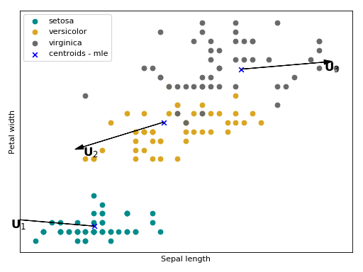
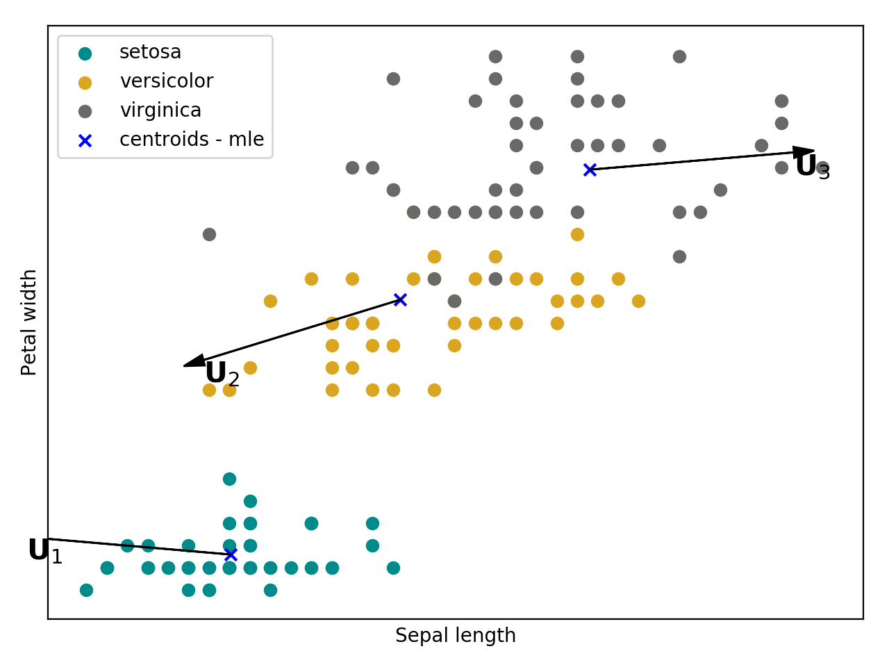
Inter-Session Variability (ISV) modeling [3] [2] is a session variability modeling technique built on top of the Gaussian mixture modeling approach. It hypothesizes that within-class variations are embedded in a linear subspace in the GMM means subspace and these variations can be suppressed by an offset w.r.t each mean during the MAP adaptation.
In this generative model each sample is assumed to have been generated by a GMM mean supervector with the following shape: \(\mu_{i, j} = m + Ux_{i, j} + D_z{i}\), where \(m\) is our prior, \(Ux_{i, j}\) is the session offset that we want to suppress and \(D_z{i}\) is the class offset (with all session effects suppressed).
All possible sources of session variations is embedded in this matrix \(U\). Follow bellow an intuition of what is modeled with \(U\) in the Iris flower dataset. The arrows \(U_{1}\), \(U_{2}\) and \(U_{3}\) are the directions of the within class variations, with respect to each Gaussian component, that will be suppressed a posteriori.
(Source code, png, hires.png, pdf)

The ISV statistical model is stored in this container
bob.learn.em.ISVBase and the training is performed by
bob.learn.em.ISVTrainer. The snippet bellow shows how to train a
Intersession variability modeling.
 >>> import bob.learn.em
 >>> import numpy
 >>> numpy.random.seed(10)
 >>>
 >>> # Generating some fake data
 >>> data_class1 = numpy.random.normal(0, 0.5, (10, 3))
 >>> data_class2 = numpy.random.normal(-0.2, 0.2, (10, 3))
 >>> data = [data_class1, data_class2]

 >>> # Creating a fake prior with 2 gaussians of dimension 3
 >>> prior_gmm = bob.learn.em.GMMMachine(2, 3)
 >>> prior_gmm.means = numpy.vstack((numpy.random.normal(0, 0.5, (1, 3)),
 ...                                 numpy.random.normal(1, 0.5, (1, 3))))
 >>> # All nice and round diagonal covariance
 >>> prior_gmm.variances = numpy.ones((2, 3)) * 0.5
 >>> prior_gmm.weights = numpy.array([0.3, 0.7])
 >>> # The input the the ISV Training is the statistics of the GMM
 >>> gmm_stats_per_class = []
 >>> for d in data:
 ...   stats = []
 ...   for i in d:
 ...     gmm_stats_container = bob.learn.em.GMMStats(2, 3)
 ...     prior_gmm.acc_statistics(i, gmm_stats_container)
 ...     stats.append(gmm_stats_container)
 ...   gmm_stats_per_class.append(stats)

 >>> # Finally doing the ISV training
 >>> subspace_dimension_of_u = 2
 >>> relevance_factor = 4
 >>> isvbase = bob.learn.em.ISVBase(prior_gmm, subspace_dimension_of_u)
 >>> trainer = bob.learn.em.ISVTrainer(relevance_factor)
 >>> bob.learn.em.train(trainer, isvbase, gmm_stats_per_class,
 ...                    max_iterations=50)
 >>> # Printing the session offset w.r.t each Gaussian component
 >>> print(isvbase.u)
   [[-0.01  -0.027]
   [-0.002 -0.004]
   [ 0.028  0.074]
   [ 0.012  0.03 ]
   [ 0.033  0.085]
   [ 0.046  0.12 ]]
Joint Factor Analysis
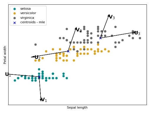
Joint Factor Analysis (JFA) [1] [2] is an extension of ISV. Besides the within-class assumption (modeled with \(U\)), it also hypothesize that between class variations are embedded in a low rank rectangular matrix \(V\). In the supervector notation, this modeling has the following shape: \(\mu_{i, j} = m + Ux_{i, j} + Vy_{i} + D_z{i}\).
Follow bellow an intuition of what is modeled with \(U\) and \(V\) in the Iris flower dataset. The arrows \(V_{1}\), \(V_{2}\) and \(V_{3}\) are the directions of the between class variations with respect to each Gaussian component that will be added a posteriori.
(Source code, png, hires.png, pdf)
The JFA statistical model is stored in this container
bob.learn.em.JFABase and the training is performed by
bob.learn.em.JFATrainer. The snippet bellow shows how to train a
Intersession variability modeling.
 >>> import bob.learn.em
 >>> import numpy
 >>> numpy.random.seed(10)
 >>>
 >>> # Generating some fake data
 >>> data_class1 = numpy.random.normal(0, 0.5, (10, 3))
 >>> data_class2 = numpy.random.normal(-0.2, 0.2, (10, 3))
 >>> data = [data_class1, data_class2]

 >>> # Creating a fake prior with 2 Gaussians of dimension 3
 >>> prior_gmm = bob.learn.em.GMMMachine(2, 3)
 >>> prior_gmm.means = numpy.vstack((numpy.random.normal(0, 0.5, (1, 3)),
 ...                                 numpy.random.normal(1, 0.5, (1, 3))))
 >>> # All nice and round diagonal covariance
 >>> prior_gmm.variances = numpy.ones((2, 3)) * 0.5
 >>> prior_gmm.weights = numpy.array([0.3, 0.7])
 >>>
 >>> # The input the the JFA Training is the statistics of the GMM
 >>> gmm_stats_per_class = []
 >>> for d in data:
 ...   stats = []
 ...   for i in d:
 ...     gmm_stats_container = bob.learn.em.GMMStats(2, 3)
 ...     prior_gmm.acc_statistics(i, gmm_stats_container)
 ...     stats.append(gmm_stats_container)
 ...   gmm_stats_per_class.append(stats)
 >>>
 >>> # Finally doing the JFA training
 >>> subspace_dimension_of_u = 2
 >>> subspace_dimension_of_v = 2
 >>> relevance_factor = 4
 >>> jfabase = bob.learn.em.JFABase(prior_gmm, subspace_dimension_of_u,
 ...                                subspace_dimension_of_v)
 >>> trainer = bob.learn.em.JFATrainer()
 >>> bob.learn.em.train_jfa(trainer, jfabase, gmm_stats_per_class,
 ...                        max_iterations=50)

 >>> # Printing the session offset w.r.t each Gaussian component
 >>> print(jfabase.v)
  [[ 0.003 -0.006]
   [ 0.041 -0.084]
   [-0.261  0.53 ]
   [-0.252  0.51 ]
   [-0.387  0.785]
   [-0.36   0.73 ]]
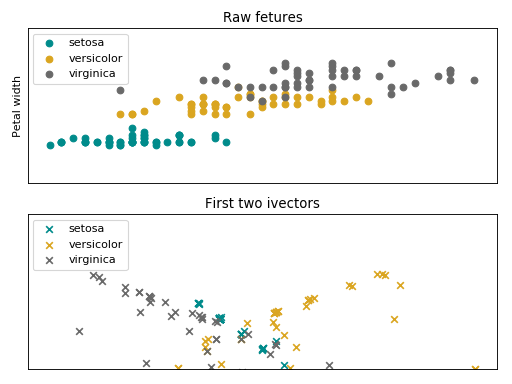
Total variability Modelling
Total Variability (TV) modeling [4] is a front-end initially introduced for
speaker recognition, which aims at describing samples by vectors of low
dimensionality called i-vectors. The model consists of a subspace \(T\)
and a residual diagonal covariance matrix \(\Sigma\), that are then used to
extract i-vectors, and is built upon the GMM approach. In the supervector
notation this modeling has the following shape: \(\mu = m + Tv\).
Follow bellow an intuition of the data from the Iris flower dataset, embedded in the iVector space.
(Source code, png, hires.png, pdf)
The iVector statistical model is stored in this container
bob.learn.em.IVectorMachine and the training is performed by
bob.learn.em.IVectorTrainer. The snippet bellow shows how to train
a Total variability modeling.
 >>> import bob.learn.em
 >>> import numpy
 >>> numpy.random.seed(10)
 >>>
 >>> # Generating some fake data
 >>> data_class1 = numpy.random.normal(0, 0.5, (10, 3))
 >>> data_class2 = numpy.random.normal(-0.2, 0.2, (10, 3))
 >>> data = [data_class1, data_class2]
 >>>
 >>> # Creating a fake prior with 2 gaussians of dimension 3
 >>> prior_gmm = bob.learn.em.GMMMachine(2, 3)
 >>> prior_gmm.means = numpy.vstack((numpy.random.normal(0, 0.5, (1, 3)),
 ...                                 numpy.random.normal(1, 0.5, (1, 3))))
 >>> # All nice and round diagonal covariance
 >>> prior_gmm.variances = numpy.ones((2, 3)) * 0.5
 >>> prior_gmm.weights = numpy.array([0.3, 0.7])
 >>>
 >>> # The input the the TV Training is the statistics of the GMM
 >>> gmm_stats_per_class = []
 >>> for d in data:
 ...     for i in d:
 ...       gmm_stats_container = bob.learn.em.GMMStats(2, 3)
 ...       prior_gmm.acc_statistics(i, gmm_stats_container)
 ...       gmm_stats_per_class.append(gmm_stats_container)
 >>>
 >>> # Finally doing the TV training
 >>> subspace_dimension_of_t = 2
 >>>
 >>> ivector_trainer = bob.learn.em.IVectorTrainer(update_sigma=True)
 >>> ivector_machine = bob.learn.em.IVectorMachine(
 ...     prior_gmm, subspace_dimension_of_t, 10e-5)
 >>> # train IVector model
 >>> bob.learn.em.train(ivector_trainer, ivector_machine,
 ...                    gmm_stats_per_class, 500)
 >>>
 >>> # Printing the session offset w.r.t each Gaussian component
 >>> print(ivector_machine.t)
  [[ 0.11  -0.203]
   [-0.124  0.014]
   [ 0.296  0.674]
   [ 0.447  0.174]
   [ 0.425  0.583]
   [ 0.394  0.794]]
Linear Scoring
In MAP adaptation, ISV and JFA a traditional way to do scoring is via the log-likelihood ratio between the adapted model and the prior as the following:
(with \(\Theta\) varying for each approach).
A simplification proposed by [Glembek2009], called linear scoring, approximate this ratio using a first order Taylor series as the following:
where \(\mu\) is the the GMM mean supervector (of the prior and the adapted
model), \(\sigma\) is the variance, supervector, \(f\) is the first
order GMM statistics (bob.learn.em.GMMStats.sum_px) and
\(U_x\), is possible channel offset (ISV).
This scoring technique is implemented in bob.learn.em.linear_scoring().
The snippet bellow shows how to compute scores using this approximation.
>>> import bob.learn.em
>>> import numpy
>>> # Defining a fake prior
>>> prior_gmm = bob.learn.em.GMMMachine(3, 2)
>>> prior_gmm.means = numpy.array([[1, 1], [2, 2.1], [3, 3]])
>>> # Defining a fake prior
>>> adapted_gmm = bob.learn.em.GMMMachine(3,2)
>>> adapted_gmm.means = numpy.array([[1.5, 1.5], [2.5, 2.5], [2, 2]])
>>> # Defining an input
>>> input = numpy.array([[1.5, 1.5], [1.6, 1.6]])
>>> #Accumulating statistics of the GMM
>>> stats = bob.learn.em.GMMStats(3, 2)
>>> prior_gmm.acc_statistics(input, stats)
>>> score = bob.learn.em.linear_scoring(
...     [adapted_gmm], prior_gmm, [stats], [],
...     frame_length_normalisation=True)
>>> print(score)
 [[ 0.254]]
Probabilistic Linear Discriminant Analysis (PLDA)
Probabilistic Linear Discriminant Analysis [5] is a probabilistic model that incorporates components describing both between-class and within-class variations. Given a mean \(\mu\), between-class and within-class subspaces \(F\) and \(G\) and residual noise \(\epsilon\) with zero mean and diagonal covariance matrix \(\Sigma\), the model assumes that a sample \(x_{i,j}\) is generated by the following process:
An Expectation-Maximization algorithm can be used to learn the parameters of
this model \(\mu\), \(F\) \(G\) and \(\Sigma\). As these
parameters can be shared between classes, there is a specific container class
for this purpose, which is bob.learn.em.PLDABase. The process is
described in detail in [6].
Let us consider a training set of two classes, each with 3 samples of dimensionality 3.
>>> data1 = numpy.array(
...     [[3,-3,100],
...      [4,-4,50],
...      [40,-40,150]], dtype=numpy.float64)
>>> data2 = numpy.array(
...     [[3,6,-50],
...      [4,8,-100],
...      [40,79,-800]], dtype=numpy.float64)
>>> data = [data1,data2]
Learning a PLDA model can be performed by instantiating the class
bob.learn.em.PLDATrainer, and calling the
bob.learn.em.train() method.
>>> # This creates a PLDABase container for input feature of dimensionality
>>> # 3 and with subspaces F and G of rank 1 and 2, respectively.
>>> pldabase = bob.learn.em.PLDABase(3,1,2)

>>> trainer = bob.learn.em.PLDATrainer()
>>> bob.learn.em.train(trainer, pldabase, data, max_iterations=10)
Once trained, this PLDA model can be used to compute the log-likelihood of a
set of samples given some hypothesis. For this purpose, a
bob.learn.em.PLDAMachine should be instantiated. Then, the
log-likelihood that a set of samples share the same latent identity variable
\(h_{i}\) (i.e. the samples are coming from the same identity/class) is
obtained by calling the
bob.learn.em.PLDAMachine.compute_log_likelihood() method.
>>> plda = bob.learn.em.PLDAMachine(pldabase)
>>> samples = numpy.array(
...     [[3.5,-3.4,102],
...      [4.5,-4.3,56]], dtype=numpy.float64)
>>> loglike = plda.compute_log_likelihood(samples)
If separate models for different classes need to be enrolled, each of them with
a set of enrollment samples, then, several instances of
bob.learn.em.PLDAMachine need to be created and enrolled using
the bob.learn.em.PLDATrainer.enroll() method as follows.
>>> plda1 = bob.learn.em.PLDAMachine(pldabase)
>>> samples1 = numpy.array(
...     [[3.5,-3.4,102],
...      [4.5,-4.3,56]], dtype=numpy.float64)
>>> trainer.enroll(plda1, samples1)
>>> plda2 = bob.learn.em.PLDAMachine(pldabase)
>>> samples2 = numpy.array(
...     [[3.5,7,-49],
...      [4.5,8.9,-99]], dtype=numpy.float64)
>>> trainer.enroll(plda2, samples2)
Afterwards, the joint log-likelihood of the enrollment samples and of one or several test samples can be computed as previously described, and this separately for each model.
>>> sample = numpy.array([3.2,-3.3,58], dtype=numpy.float64)
>>> l1 = plda1.compute_log_likelihood(sample)
>>> l2 = plda2.compute_log_likelihood(sample)
In a verification scenario, there are two possible hypotheses:
- \(x_{test}\) and \(x_{enroll}\) share the same class.
- \(x_{test}\) and \(x_{enroll}\) are from different classes.
Using the methods bob.learn.em.PLDAMachine.log_likelihood_ratio() or
its alias __call__ function, the corresponding log-likelihood ratio will be
computed, which is defined in more formal way by:
\(s = \ln(P(x_{test},x_{enroll})) - \ln(P(x_{test})P(x_{enroll}))\)
>>> s1 = plda1(sample)
>>> s2 = plda2(sample)
Score Normalization
Score normalization aims to compensate statistical variations in output scores due to changes in the conditions across different enrollment and probe samples. This is achieved by scaling distributions of system output scores to better facilitate the application of a single, global threshold for authentication.
Bob has implemented 3 different strategies to normalize scores and these strategies are presented in the next subsections.
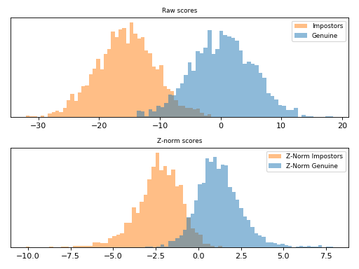
Z-Norm
Given a score \(s_i\), Z-Norm [Auckenthaler2000] and [Mariethoz2005] (zero-normalization) scales this value by the mean (\(\mu\)) and standard deviation (\(\sigma\)) of an impostor score distribution. This score distribution can be computed before hand and it is defined as the following.
This scoring technique is implemented in bob.learn.em.znorm(). Follow
bellow an example of score normalization using bob.learn.em.znorm().
import matplotlib.pyplot as plt
import bob.learn.em
import numpy
numpy.random.seed(10)


n_clients = 10
n_scores_per_client = 200

# Defining some fake scores for genuines and impostors
impostor_scores = numpy.random.normal(-15.5,
                                      5, (n_scores_per_client, n_clients))
genuine_scores = numpy.random.normal(0.5, 5, (n_scores_per_client, n_clients))

# Defining the scores for the statistics computation
z_scores = numpy.random.normal(-5., 5, (n_scores_per_client, n_clients))

# Z - Normalizing
z_norm_impostors = bob.learn.em.znorm(impostor_scores, z_scores)
z_norm_genuine = bob.learn.em.znorm(genuine_scores, z_scores)

# PLOTTING
figure = plt.subplot(2, 1, 1)
ax = figure.axes
plt.title("Raw scores", fontsize=8)
plt.hist(impostor_scores.reshape(n_scores_per_client * n_clients),
         label='Impostors', normed=True,
         color='C1', alpha=0.5, bins=50)
plt.hist(genuine_scores.reshape(n_scores_per_client * n_clients),
         label='Genuine', normed=True,
         color='C0', alpha=0.5, bins=50)
plt.legend(fontsize=8)
plt.yticks([], [])


figure = plt.subplot(2, 1, 2)
ax = figure.axes
plt.title("Z-norm scores", fontsize=8)
plt.hist(z_norm_impostors.reshape(n_scores_per_client * n_clients),
         label='Z-Norm Impostors', normed=True,
         color='C1', alpha=0.5, bins=50)
plt.hist(z_norm_genuine.reshape(n_scores_per_client * n_clients),
         label='Z-Norm Genuine', normed=True,
         color='C0', alpha=0.5, bins=50)
plt.yticks([], [])
plt.legend(fontsize=8)

plt.tight_layout()
plt.show()
(Source code, png, hires.png, pdf)

Note
Observe how the scores were scaled in the plot above.
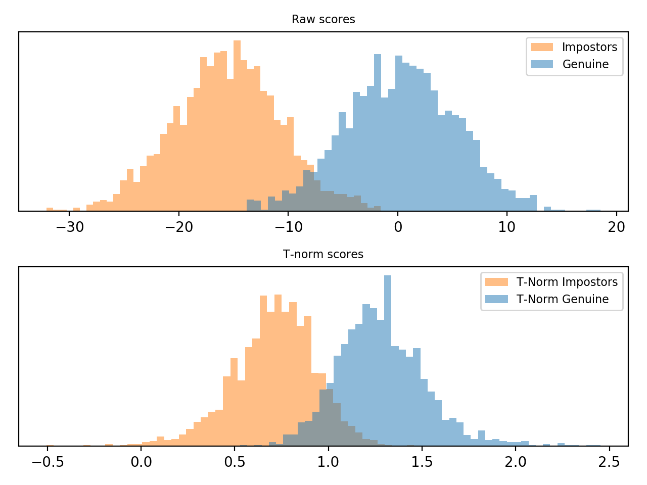
T-Norm
T-norm [Auckenthaler2000] and [Mariethoz2005] (Test-normalization) operates in a probe-centric manner. If in the Z-Norm \(\mu\) and \(\sigma\) are estimated using an impostor set of models and its scores, the t-norm computes these statistics using the current probe sample against at set of models in a co-hort \(\Theta_{c}\). A co-hort can be any semantic organization that is sensible to your recognition task, such as sex (male and females), ethnicity, age, etc and is defined as the following.
where, \(s_i\) is \(P(x_i | \Theta)\) (the score given the claimed model), \(\mu = \frac{ \sum\limits_{i=0}^{N} P(x_i | \Theta_{c}) }{N}\) (\(\Theta_{c}\) are the models of one co-hort) and \(\sigma\) is the standard deviation computed using the same criteria used to compute \(\mu\).
This scoring technique is implemented in bob.learn.em.tnorm(). Follow
bellow an example of score normalization using bob.learn.em.tnorm().
import matplotlib.pyplot as plt
import bob.learn.em
import numpy
numpy.random.seed(10)

n_clients = 10
n_scores_per_client = 200

# Defining some fake scores for genuines and impostors
impostor_scores = numpy.random.normal(-15.5,
                                      5, (n_scores_per_client, n_clients))
genuine_scores = numpy.random.normal(0.5, 5, (n_scores_per_client, n_clients))

# Defining the scores for the statistics computation
t_scores = numpy.random.normal(-5., 5, (n_scores_per_client, n_clients))

# T - Normalizing
t_norm_impostors = bob.learn.em.tnorm(impostor_scores, t_scores)
t_norm_genuine = bob.learn.em.tnorm(genuine_scores, t_scores)

# PLOTTING
figure = plt.subplot(2, 1, 1)
ax = figure.axes
plt.title("Raw scores", fontsize=8)
plt.hist(impostor_scores.reshape(n_scores_per_client * n_clients),
         label='Impostors', normed=True,
         color='C1', alpha=0.5, bins=50)
plt.hist(genuine_scores.reshape(n_scores_per_client * n_clients),
         label='Genuine', normed=True,
         color='C0', alpha=0.5, bins=50)
plt.legend(fontsize=8)
plt.yticks([], [])


figure = plt.subplot(2, 1, 2)
ax = figure.axes
plt.title("T-norm scores", fontsize=8)
plt.hist(t_norm_impostors.reshape(n_scores_per_client * n_clients),
         label='T-Norm Impostors', normed=True,
         color='C1', alpha=0.5, bins=50)
plt.hist(t_norm_genuine.reshape(n_scores_per_client * n_clients),
         label='T-Norm Genuine', normed=True,
         color='C0', alpha=0.5, bins=50)
plt.legend(fontsize=8)
plt.yticks([], [])

plt.tight_layout()
plt.show()
(Source code, png, hires.png, pdf)
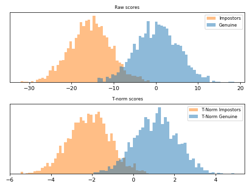
Note
T-norm introduces extra computation during scoring, as the probe samples need to be compared to each cohort model in order to have \(\mu\) and \(\sigma\).
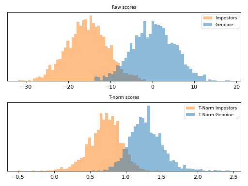
ZT-Norm
ZT-Norm [Auckenthaler2000] and [Mariethoz2005] consists in the application of
Z-Norm followed by a T-Norm and it is implemented
in bob.learn.em.ztnorm().
Follow bellow an example of score normalization using
bob.learn.em.ztnorm().
import matplotlib.pyplot as plt
import bob.learn.em
import numpy
numpy.random.seed(10)

n_clients = 10
n_scores_per_client = 200

# Defining some fake scores for genuines and impostors
impostor_scores = numpy.random.normal(-15.5,
                                      5, (n_scores_per_client, n_clients))
genuine_scores = numpy.random.normal(0.5, 5, (n_scores_per_client, n_clients))

# Defining the scores for the statistics computation
z_scores = numpy.random.normal(-5., 5, (n_scores_per_client, n_clients))
t_scores = numpy.random.normal(-6., 5, (n_scores_per_client, n_clients))

# T-normalizing the Z-scores
zt_scores = bob.learn.em.tnorm(z_scores, t_scores)

# ZT - Normalizing
zt_norm_impostors = bob.learn.em.ztnorm(
    impostor_scores, z_scores, t_scores, zt_scores)
zt_norm_genuine = bob.learn.em.ztnorm(
    genuine_scores, z_scores, t_scores, zt_scores)

# PLOTTING
figure = plt.subplot(2, 1, 1)
ax = figure.axes
plt.title("Raw scores", fontsize=8)
plt.hist(impostor_scores.reshape(n_scores_per_client * n_clients),
         label='Impostors', normed=True,
         color='C1', alpha=0.5, bins=50)
plt.hist(genuine_scores.reshape(n_scores_per_client * n_clients),
         label='Genuine', normed=True,
         color='C0', alpha=0.5, bins=50)
plt.legend(fontsize=8)
plt.yticks([], [])


figure = plt.subplot(2, 1, 2)
ax = figure.axes
plt.title("T-norm scores", fontsize=8)
plt.hist(zt_norm_impostors.reshape(n_scores_per_client * n_clients),
         label='T-Norm Impostors', normed=True,
         color='C1', alpha=0.5, bins=50)
plt.hist(zt_norm_genuine.reshape(n_scores_per_client * n_clients),
         label='T-Norm Genuine', normed=True,
         color='C0', alpha=0.5, bins=50)
plt.legend(fontsize=8)
plt.yticks([], [])

plt.tight_layout()
plt.show()
(Source code, png, hires.png, pdf)

Note
Observe how the scores were scaled in the plot above.
| [1] | http://dx.doi.org/10.1109/TASL.2006.881693 |
| [2] | (1, 2) http://publications.idiap.ch/index.php/publications/show/2606 |
| [3] | http://dx.doi.org/10.1016/j.csl.2007.05.003 |
| [4] | http://dx.doi.org/10.1109/TASL.2010.2064307 |
| [5] | http://dx.doi.org/10.1109/ICCV.2007.4409052 |
| [6] | http://doi.ieeecomputersociety.org/10.1109/TPAMI.2013.38 |
| [7] | http://en.wikipedia.org/wiki/K-means_clustering |
| [8] | (1, 2, 3) http://en.wikipedia.org/wiki/Expectation-maximization_algorithm |
| [9] | http://en.wikipedia.org/wiki/Maximum_likelihood |
| [10] | http://en.wikipedia.org/wiki/Maximum_a_posteriori_estimation |