Image Processing Guide
Introduction
The basic operations on images are the affine image conversions like image scaling, rotation, and cutting. For most of the operations, two ways of executing the functions exist. The easier API simply returns the processed image, but the second version accepts input and output objects (to allow memory reuse).
Scaling images
To compute a scaled version of the image, simply create the image at the desired scale. For instance, in the example below an image is up-scaled by first creating the image and then initializing the larger image:
>>> A = numpy.array( [ [1, 2, 3], [4, 5, 6] ], dtype = numpy.uint8 ) # A small image of size 2x3
>>> print(A)
[[1 2 3]
 [4 5 6]]
>>> B = numpy.ndarray( (3, 5), dtype = numpy.float64 )               # A larger image of size 3x5
the bob.ip.base.scale() function of Bob is then called to up-scale the image:
>>> bob.ip.base.scale(A, B)
>>> numpy.allclose(B, [[ 1.,1.5, 2., 2.5,  3.],[ 2.5, 3.,3.5, 4., 4.5],[ 4.,4.5, 5., 5.5,6. ]])
True
which bi-linearly interpolates image A to image B. Of course, scaling factors can be different in horizontal and vertical direction:
>>> C = numpy.ndarray( (2, 5), dtype = numpy.float64 )
>>> bob.ip.base.scale(A, C)
>>> numpy.allclose(C, [[1., 1.5,  2., 2.5, 3.],[4., 4.5, 5., 5.5, 6. ]])
True
Rotating images
The rotation of an image is slightly more difficult since the resulting image
size has to be computed in advance. To facilitate this there is a function
bob.ip.base.rotated_output_shape() which can be used:
>>> A = numpy.array( [ [1, 2, 3], [4, 5, 6] ], dtype = numpy.uint8 ) # A small image of size 3x3
>>> print(A)
[[1 2 3]
 [4 5 6]]
>>> rotated_shape = bob.ip.base.rotated_output_shape( A, 90 )
>>> print(rotated_shape)
(3, 2)
After the creation of the image in the desired size, the
bob.ip.base.rotate() function can be executed:
>>> A_rotated = numpy.ndarray( rotated_shape, dtype = numpy.float64 ) # A small image of rotated size
>>> bob.ip.base.rotate(A, A_rotated, 90)      # execute the rotation
>>> numpy.allclose(A_rotated, [[ 3.,  6.],[ 2.,  5.],[ 1.,  4.]])
True
Complex image operations
Complex image operations are usually wrapped up by classes. The usual work flow is to first generate an object of the desired class, specifying parameters that are independent on the images to operate, and to second use the class on images. Usually, objects that perform image operations have the __call__ function overloaded, so that one simply can use it as if it were functions. Below we provide some examples.
Image filtering
One simple example of image filtering is to apply a Gaussian blur filter to an image.
This can be easily done by first creating an object of the bob.ip.base.Gaussian class:
>>> filter = bob.ip.base.Gaussian(sigma = (3., 3.), radius = (5, 5))
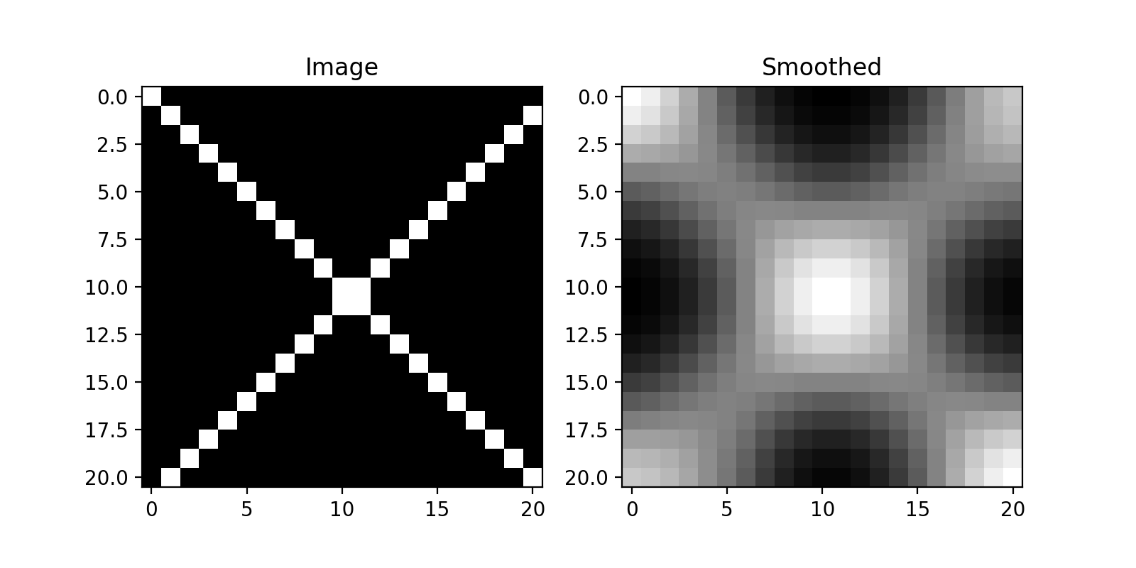
Now, let’s see what happens to a small test image:
import bob.ip.base
import numpy
import math

# create test image
image = numpy.zeros((21,21))
for i in range(21):
  image[i,i] = 255
  image[-i,i] = 255

# perform Gaussian filtering
gaussian = bob.ip.base.Gaussian(sigma = (3., 3.), radius = (5, 5))
smoothed = gaussian(image)

# plot results
from matplotlib import pyplot
pyplot.figure(figsize=(8,4))
pyplot.subplot(121) ; pyplot.imshow(image, cmap='gray')    ; pyplot.title('Image')
pyplot.subplot(122) ; pyplot.imshow(smoothed, cmap='gray') ; pyplot.title('Smoothed')
pyplot.show()
(Source code, png, hires.png, pdf)
The image of the cross has now been nicely smoothed.
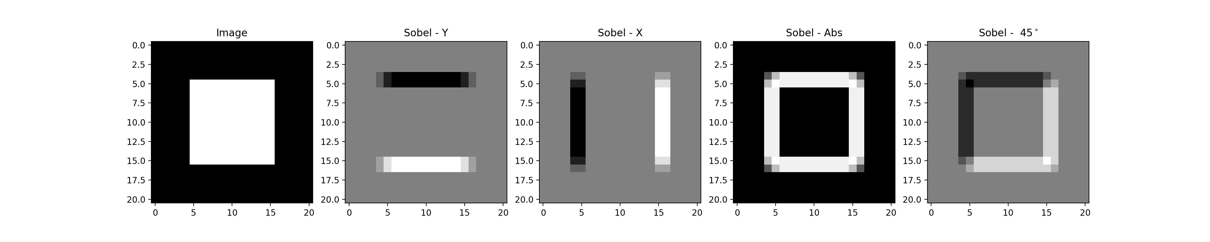
A second example uses Sobel filters to extract edges from an image. Two types of Sobel filters exist: The vertical filter \(S_y\) and the horizontal filter \(S_x\):
Both filters can be applied at the same time using the bob.ip.base.sobel() function, where the result of \(S_y\) will be put to the first layer and \(S_x\) to the second layer.
>>> image = numpy.zeros((21,21))
>>> image[5:16, 5:16] = 1
>>> sobel = bob.ip.base.sobel(image)
>>> sobel.shape
(2, 21, 21)
Interestingly, the vertical filter \(S_y\) extracts horizontal edges, while the \(S_x\) extracts vertical edges. In fact, the vector \((s_y, s_x)^T\) contains the gradient information at a given location in the image. To get the direction-independent strength of the edge at that point, simply compute the Euclidean length of the gradient. To compute rotation-dependent results, use the rotation matrix on the gradient vector.
import bob.ip.base
import numpy
import math

# create test image
image = numpy.zeros((21,21))
image[5:16, 5:16] = 1

# perform Sobel filtering
sobel = bob.ip.base.sobel(image)

# compute direction-independent and direction-dependent results
abs_sobel = numpy.sqrt(numpy.square(sobel[0]) + numpy.square(sobel[1]))
angle = 45.
rot_sobel = math.sin(angle*math.pi/180) * sobel[0] + math.cos(angle*math.pi/180) * sobel[1]

# plot results
from matplotlib import pyplot
pyplot.figure(figsize=(20,4))
pyplot.subplot(151) ; pyplot.imshow(image, cmap='gray')     ; pyplot.title('Image')
pyplot.subplot(152) ; pyplot.imshow(sobel[0], cmap='gray')  ; pyplot.title('Sobel - Y')
pyplot.subplot(153) ; pyplot.imshow(sobel[1], cmap='gray')  ; pyplot.title('Sobel - X')
pyplot.subplot(154) ; pyplot.imshow(abs_sobel, cmap='gray') ; pyplot.title('Sobel - Abs')
pyplot.subplot(155) ; pyplot.imshow(rot_sobel, cmap='gray') ; pyplot.title('Sobel - %3.0f$^\circ$'%angle)
pyplot.show()
(Source code, png, hires.png, pdf)

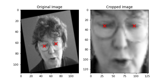
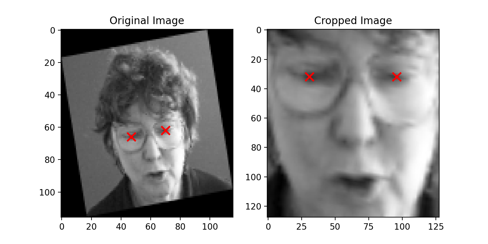
Normalizing face images according to eye positions
For many face biometrics applications, for instance face recognition, the images are
geometrically normalized according to the eye positions. In such a case, the
first thing to do is to create an object of the bob.ip.base.FaceEyesNorm class defining the image
properties of the geometrically normalized image (that will be generated when
applying the object):
>>> face_eyes_norm = bob.ip.base.FaceEyesNorm(eyes_distance = 65, crop_size = (128, 128), eyes_center = (32, 63.5))
Now, we have set up our object to generate images of size (128, 128) that will put the left eye at the pixel position (32, 31) and the right eye at the position (32, 96). Afterwards, this object is used to geometrically normalize the face, given the eye positions in the original face image. Note that the left eye usually has a higher x-coordinate than the right eye:
>>> face_image = bob.io.base.load( image_path )
>>> cropped_image = numpy.ndarray( (128, 128), dtype = numpy.float64 )
>>> face_eyes_norm( face_image, cropped_image, right_eye = (66, 47), left_eye = (62, 70) )
Now, let’s have a look at the original and normalized face:
import numpy
import math
import bob.io.base
import bob.ip.base
from bob.io.base.test_utils import datafile

# load a test image
face_image = bob.io.base.load(datafile('image_r10.hdf5', 'bob.ip.base', 'data/affine'))

# create FaceEyesNorm class
face_eyes_norm = bob.ip.base.FaceEyesNorm(eyes_distance = 65, crop_size = (128, 128), eyes_center = (32, 63.5))

# normalize image
normalized_image = face_eyes_norm( face_image, right_eye = (66, 47), left_eye = (62, 70) )

# plot results, including eye locations in original and normalized image
from matplotlib import pyplot
pyplot.figure(figsize=(8,4))
pyplot.subplot(121) ; pyplot.imshow(face_image, cmap='gray')       ; pyplot.plot([47, 70], [66, 62], 'rx', ms=10, mew=2); pyplot.axis('tight'); pyplot.title('Original Image')
pyplot.subplot(122) ; pyplot.imshow(normalized_image, cmap='gray') ; pyplot.plot([31, 96], [32, 32], 'rx', ms=10, mew=2); pyplot.axis('tight'); pyplot.title('Cropped Image')
pyplot.show()
(Source code, png, hires.png, pdf)

Simple feature extraction
Some simple feature extraction functionality is also included in the
bob.ip.base module. Here is some simple example, how to extract
local binary patterns (LBP) with 8 neighbors from an image:
>>> lbp_extractor = bob.ip.base.LBP(8)
You can either get the LBP feature for a single point by specifying the position:
>>> lbp_local = lbp_extractor ( cropped_image, (69, 62) )
>>> # print the binary representation of the LBP
>>> print(bin ( lbp_local ))
0b1111000
or you can extract the LBP features for all pixels in the image. In this case
you need to get the required shape of the output image using the bob.ip.base.LBP feature extractor:
>>> lbp_output_image_shape = lbp_extractor.lbp_shape(cropped_image)
>>> print(lbp_output_image_shape)
(126, 126)
>>> lbp_output_image = numpy.ndarray ( lbp_output_image_shape, dtype = numpy.uint16 )
>>> lbp_extractor ( cropped_image,  lbp_output_image )
>>> # print the binary representation of the pixel at the same location as above;
>>> # note that the index is shifted by 1 since the lbp image is smaller than the original
>>> print(bin ( lbp_output_image [ 68, 61 ] ))
0b1111000
LBP-TOP extraction
LBP-TOP [Zhao2007] extraction for temporal texture analysis.
>>> import bob.ip.base
>>> import numpy
>>> numpy.random.seed(10)
>>> #Defining the lbp operator for each plane
>>> lbp_xy = bob.ip.base.LBP(8,1)
>>> lbp_xt = bob.ip.base.LBP(8,1)
>>> lbp_yt = bob.ip.base.LBP(8,1)
>>> lbptop = bob.ip.base.LBPTop(lbp_xy, lbp_xt, lbp_yt)
Defining the test 3D image and creating the containers for the outputs in each plane
>>> img3d = (numpy.random.rand(3,5,5)*100).astype('uint16')
>>> t = int(max(lbp_xt.radius, lbp_yt.radius))
>>> w = int(img3d.shape[1] - lbp_xy.radii[0]*2)
>>> h = int(img3d.shape[2] - lbp_xy.radii[1]*2)
>>> output_xy = numpy.zeros((t,w,h),dtype='uint16')
>>> output_xt = numpy.zeros((t,w,h),dtype='uint16')
>>> output_yt = numpy.zeros((t,w,h),dtype='uint16')
Extracting the bins for each plane
>>> lbptop(img3d,output_xy, output_xt, output_yt)
>>> print(output_xy)
[[[ 89   0 235]
[255  72 255]
[ 40  95   2]]]
>>> print(output_xt)
[[[ 55   2 135]
[223 130 119]
[  0 253  64]]]
>>> print(output_yt)
[[[ 45   0 173]
[247   1 255]
[130 127  64]]]