A Complete Application: Analysis of the Fisher Iris Dataset
The Iris flower data set or Fisher’s Iris data set is a multivariate data set introduced by Sir Ronald Aylmer Fisher (1936) as an example of discriminant analysis. It is sometimes called Anderson’s Iris data set because Edgar Anderson collected the data to quantify the morphologic variation of Iris flowers of three related species. The dataset consists of 50 samples from each of three species of Iris flowers (Iris setosa, Iris virginica and Iris versicolor). Four features were measured from each sample, they are the length and the width of sepal and petal, in centimeters. Based on the combination of the four features, Fisher developed a linear discriminant model to distinguish the species from each other.
In this example, we collect bits and pieces of the previous tutorials and build a complete example that discriminates Iris species based on Bob.
Note
This example will consider all 3 classes for the LDA training. This is not what Fisher did in his paper [Fisher1936] . In that work Fisher did the right thing only for the first 2-class problem (setosa versus versicolor). You can reproduce the 2-class LDA using bob’s LDA training system without problems. When inserting the virginica class, Fisher decides for a different metric (4vi + ve - 5se) and solves for the matrices in the last row of Table VIII.
This is OK, but does not generalize the method proposed in the beginning of his paper. Results achieved by the generalized LDA method [Duda1973] will not match Fisher’s result on that last table, be aware. That being said, the final histogram presented on that paper looks quite similar to the one produced by this script, showing that Fisher’s solution was a good approximation for the generalized LDA implementation available in Bob.
| [Fisher1936] | R. A. FISHER, The Use of Multiple Measurements in Taxonomic Problems, Annals of Eugenics, pp. 179-188, 1936 |
| [Duda1973] | R.O. Duda and P.E. Hart, Pattern Classification and Scene Analysis, (Q327.D83) John Wiley & Sons. ISBN 0-471-22361-1. 1973 (See page 218). |
Training a bob.machine.LinearMachine with LDA
Creating a bob.learn.linear.Machine to perform Linear Discriminant Analysis on the Iris dataset involves using the bob.learn.linear.FisherLDATrainer:
>>> import bob.db.iris
>>> import bob.learn.linear
>>> trainer = bob.learn.linear.FisherLDATrainer()
>>> data = bob.db.iris.data()
>>> machine, unused_eigen_values = trainer.train(data.values())
>>> machine
<bob.learn.linear.Machine float64@(4, 2)>
That is it! The returned bob.learn.linear.Machine is now setup to perform LDA on the Iris data set. A few things should be noted:
- The returned bob.learn.linear.Machine represents the linear projection of the input features to a new 3D space which maximizes the between-class scatter and minimizes the within-class scatter. In other words, the internal matrix \mathbf{W} is 4-by-2. The projections are calculated internally using Singular Value Decomposition (SVD). The first projection (first row of \mathbf{W} corresponds to the highest eigenvalue resulting from the decomposition, the second, the second highest, and so on;
- The trainer also returns the eigenvalues generated after the SVD for our LDA implementation, in case you would like to use them. For this example, we just discard this information.
Looking at the first LDA component
To reproduce Fisher’s results, we must pass the data through the created machine:
>>> output = {}
>>> for key in data:
...   output[key] = machine.forward(data[key])
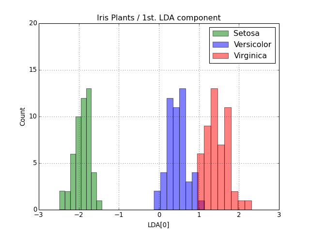
At this point the variable output contains the LDA-projected information as 2D numpy.ndarray objects. The only step missing is the visualization of the results. Fisher proposed the use of a histogram showing the separation achieved by looking at the first only. Let’s reproduce it.
>>> from matplotlib import pyplot
>>> pyplot.hist(output['setosa'][:,0], bins=8, color='green', label='Setosa', alpha=0.5)
>>> pyplot.hist(output['versicolor'][:,0], bins=8, color='blue', label='Versicolor', alpha=0.5)
>>> pyplot.hist(output['virginica'][:,0], bins=8, color='red', label='Virginica', alpha=0.5)
We can certainly throw in more decoration:
>>> pyplot.legend()
>>> pyplot.grid(True)
>>> pyplot.axis([-3,+3,0,20])
>>> pyplot.title("Iris Plants / 1st. LDA component")
>>> pyplot.xlabel("LDA[0]")
>>> pyplot.ylabel("Count")
Finally, to display the plot, do:
>>> pyplot.show()
You should see an image like this:
(Source code, png, hires.png, pdf)
Measuring performance
You can measure the performance of the system on classifying, say, Iris Virginica as compared to the other two variants. We can use the functions in bob.measure for that purpose. Let’s first find a threshold that separates this variant from the others. We choose to find the threshold at the point where the relative error rate considering both Versicolor and Setosa variants is the same as for the Virginica one.
>>> import bob.measure
>>> negatives = numpy.vstack([output['setosa'], output['versicolor']])[:,0]
>>> positives = output['virginica'][:,0]
>>> threshold= bob.measure.eer_threshold(negatives, positives)
With the threshold at hand, we can estimate the number of correctly classified negatives (or true-rejections) and positives (or true-accepts). Let’s translate that: plants from the Versicolor and Setosa variants that have the first LDA component smaller than the threshold (so called negatives at this point) and plants from the Virginica variant that have the first LDA component greater than the threshold defined (the positives). To calculate the rates, we just use bob.measure again:
>>> true_rejects = bob.measure.correctly_classified_negatives(negatives, threshold)
>>> true_accepts = bob.measure.correctly_classified_positives(positives, threshold)
From that you can calculate, for example, the number of misses at the defined threshold:
>>> sum(true_rejects)
98
>>> sum(true_accepts)
49
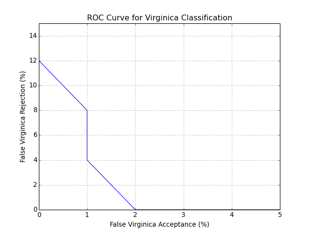
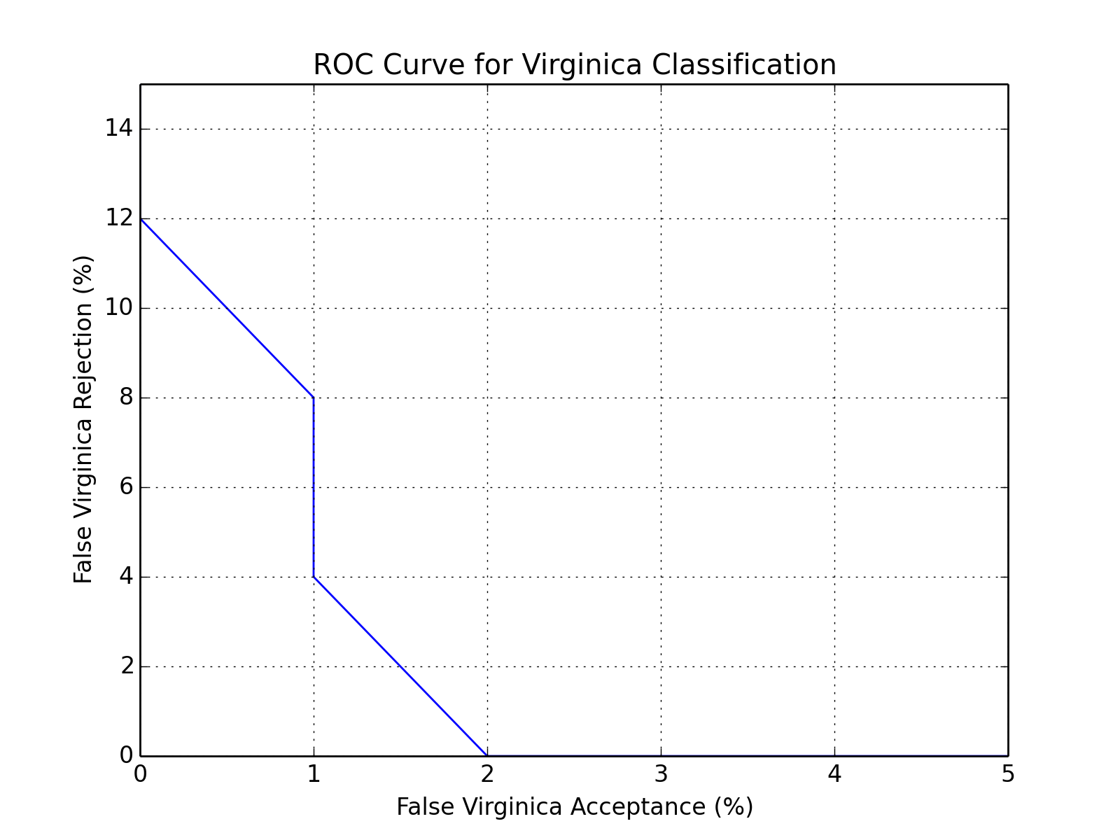
You can also plot an ROC curve. Here is the full code that will lead you to the following plot:
#!/usr/bin/env python
# Andre Anjos <andre.anjos@idiap.ch>
# Sat 24 Mar 2012 18:51:21 CET

"""Computes an ROC curve for the Iris Flower Recognition using Linear Discriminant Analysis and Bob.
"""

import bob.db.iris
import bob.learn.linear
import bob.measure
import numpy
from matplotlib import pyplot

# Training is a 3-step thing
data = bob.db.iris.data()
trainer = bob.learn.linear.FisherLDATrainer()
machine, eigen_values = trainer.train(data.values())

# A simple way to forward the data
output = {}
for key in data.keys(): output[key] = machine(data[key])

# Performance
negatives = numpy.vstack([output['setosa'], output['versicolor']])[:,0]
positives = output['virginica'][:,0]

# Plot ROC curve
bob.measure.plot.roc(negatives, positives)
pyplot.xlabel("False Virginica Acceptance (%)")
pyplot.ylabel("False Virginica Rejection (%)")
pyplot.title("ROC Curve for Virginica Classification")
pyplot.grid()
pyplot.axis([0, 5, 0, 15]) #xmin, xmax, ymin, ymax
(Source code, png, hires.png, pdf)