Executing Baseline Algorithms
The first thing you might want to do is to execute one of the vein
recognition algorithms that are implemented in bob.bio.vein.
Running Baseline Experiments
To run the baseline experiments, you can use the verify.py script by
just going to the console and typing:
$ verify.py
This script is explained in more detail in Running Biometric Recognition Experiments.
The verify.py --help option shows you, which other options you can
set.
Usually it is a good idea to have at least verbose level 2 (i.e., calling
verify.py --verbose --verbose, or the short version verify.py
-vv).
Note
Running in Parallel
To run the experiments in parallel, you can define an SGE grid or local host (multi-processing) configurations as explained in Running in Parallel.
In short, to run in the Idiap SGE grid, you can simply add the --grid
command line option, without parameters. To run experiments in parallel on
the local machine, simply add a --parallel <N> option, where <N>
specifies the number of parallel jobs you want to execute.
Database setups and baselines are encoded using
Configuration Files, all stored inside the package root, in
the directory bob/bio/vein/configurations. Documentation for each resource
is available on the section Resources.
Warning
You cannot run experiments just by executing the command line instructions described in this guide. You need first to procure yourself the raw data files that correspond to each database used here in order to correctly run experiments with those data. Biometric data is considered private data and, under EU regulations, cannot be distributed without a consent or license. You may consult our Databases resources section for checking currently supported databases and accessing download links for the raw data files.
Once the raw data files have been downloaded, particular attention should be given to the directory locations of those. Unpack the databases carefully and annotate the root directory where they have been unpacked.
Then, carefully read the Databases section of
Installation Instructions on how to correctly setup the
~/.bob_bio_databases.txt file.
Use the following keywords on the left side of the assignment (see Databases):
[YOUR_VERAFINGER_DIRECTORY] = /complete/path/to/verafinger
[YOUR_UTFVP_DIRECTORY] = /complete/path/to/utfvp
[YOUR_FV3D_DIRECTORY] = /complete/path/to/fv3d
Notice it is rather important to use the strings as described above,
otherwise bob.bio.base will not be able to correctly load your images.
Once this step is done, you can proceed with the instructions below.
In the remainder of this section we introduce baseline experiments you can readily run with this tool without further configuration. Baselines examplified in this guide were published in [TVM14].
Repeated Line-Tracking with Miura Matching
Detailed description at Repeated Line Tracking and Miura Matching.
To run the baseline on the VERA fingervein database, using the Nom
protocol, do the following:
$ verify.py verafinger rlt -vv
Tip
If you have more processing cores on your local machine and don’t want to
submit your job for SGE execution, you can run it in parallel (using 4
parallel tasks) by adding the options --parallel=4 --nice=10. Before
doing so, make sure the package gridtk is properly installed.
Optionally, you may use the parallel resource configuration which
already sets the number of parallel jobs to the number of hardware cores you
have installed on your machine (as with
multiprocessing.cpu_count()) and sets nice=10. For example:
$ verify.py verafinger rlt parallel -vv
To run on the Idiap SGE grid using our stock
io-big-48-slots-4G-memory-enabled (see
bob.bio.vein.configurations.gridio4g48) configuration, use:
$ verify.py verafinger rlt grid -vv
You may also, optionally, use the configuration resource gridio4g48,
which is just an alias of grid in this package.
This command line selects and runs the following implementations for the toolchain:
As the tool runs, you’ll see printouts that show how it advances through preprocessing, feature extraction and matching. In a 4-core machine and using 4 parallel tasks, it takes around 4 hours to process this baseline with the current code implementation.
To complete the evaluation, run the command bellow, that will output the equal error rate (EER) and plot the detector error trade-off (DET) curve with the performance:
$ bob bio metrics <path-to>/verafinger/rlt/Nom/nonorm/scores-dev --no-evaluation
[Min. criterion: EER ] Threshold on Development set `scores-dev`: 0.31835292
======  ========================
None    Development scores-dev
======  ========================
FtA     0.0%
FMR     23.6% (11388/48180)
FNMR    23.6% (52/220)
FAR     23.6%
FRR     23.6%
HTER    23.6%
======  ========================
Maximum Curvature with Miura Matching
Detailed description at Maximum Curvature and Miura Matching.
To run the baseline on the VERA fingervein database, using the Nom
protocol like above, do the following:
$ verify.py verafinger mc -vv
This command line selects and runs the following implementations for the toolchain:
In a 4-core machine and using 4 parallel tasks, it takes around 1 hour and 40 minutes to process this baseline with the current code implementation. Results we obtained:
$ bob bio metrics <path-to>/verafinger/mc/Nom/nonorm/scores-dev --no-evaluation
[Min. criterion: EER ] Threshold on Development set `scores-dev`: 7.372830e-02
======  ========================
None    Development scores-dev
======  ========================
FtA     0.0%
FMR     4.4% (2116/48180)
FNMR    4.5% (10/220)
FAR     4.4%
FRR     4.5%
HTER    4.5%
======  ========================
Wide Line Detector with Miura Matching
You can find the description of this method on the paper from Huang et al. [HDLTL10].
To run the baseline on the VERA fingervein database, using the Nom
protocol like above, do the following:
$ verify.py verafinger wld -vv
This command line selects and runs the following implementations for the toolchain:
In a 4-core machine and using 4 parallel tasks, it takes only around 5 minutes minutes to process this baseline with the current code implementation.Results we obtained:
$ bob bio metrics <path-to>/verafinger/wld/Nom/nonorm/scores-dev --no-evaluation
[Min. criterion: EER ] Threshold on Development set `scores-dev`: 2.402707e-01
======  ========================
None    Development scores-dev
======  ========================
FtA     0.0%
FMR     9.8% (4726/48180)
FNMR    10.0% (22/220)
FAR     9.8%
FRR     10.0%
HTER    9.9%
Results for other Baselines
This package may generate results for other combinations of protocols and databases. Here is a summary table for some variants (results expressed correspond to the the equal-error rate on the development set, in percentage):
Toolchain |
Vera Finger |
UTFVP |
|||
|---|---|---|---|---|---|
Feature Extractor |
Full |
B |
Nom |
1vsall |
nom |
Repeated Line Tracking |
14.6 |
13.4 |
23.6 |
3.4 |
1.4 |
Wide Line Detector |
5.8 |
5.6 |
9.9 |
2.8 |
1.9 |
Maximum Curvature |
2.5 |
1.4 |
4.5 |
0.9 |
0.4 |
In a machine with 48 cores, running these baselines took the following time (hh:mm):
Toolchain |
Vera Finger |
UTFVP |
|||
|---|---|---|---|---|---|
Feature Extractor |
Full |
B |
Nom |
1vsall |
nom |
Repeated Line Tracking |
01:16 |
00:23 |
00:23 |
12:44 |
00:35 |
Wide Line Detector |
00:07 |
00:01 |
00:01 |
02:25 |
00:05 |
Maximum Curvature |
03:28 |
00:54 |
00:59 |
58:34 |
01:48 |
Modifying Baseline Experiments
It is fairly easy to modify baseline experiments available in this package. To do so, you must copy the configuration files for the given baseline you want to modify, edit them to make the desired changes and run the experiment again.
For example, suppose you’d like to change the protocol on the Vera Fingervein
database and use the protocol full instead of the default protocol nom.
First, you identify where the configuration file sits:
$ resources.py -tc -p bob.bio.vein
- bob.bio.vein X.Y.Z @ /path/to/bob.bio.vein:
  + mc         --> bob.bio.vein.configurations.maximum_curvature
  + parallel   --> bob.bio.vein.configurations.parallel
  + rlt        --> bob.bio.vein.configurations.repeated_line_tracking
  + utfvp      --> bob.bio.vein.configurations.utfvp
  + verafinger --> bob.bio.vein.configurations.verafinger
  + wld        --> bob.bio.vein.configurations.wide_line_detector
The listing above tells the verafinger configuration file sits on the
file /path/to/bob.bio.vein/bob/bio/vein/configurations/verafinger.py. In
order to modify it, make a local copy. For example:
$ cp /path/to/bob.bio.vein/bob/bio/vein/configurations/verafinger.py verafinger_full.py
$ # edit verafinger_full.py, change the value of "protocol" to "full"
Also, don’t forget to change all relative module imports (such as from
..database.verafinger import Database) to absolute imports (e.g. from
bob.bio.vein.database.verafinger import Database). This will make the
configuration file work irrespectively of its location w.r.t. bob.bio.vein.
The final version of the modified file could look like this:
from
bob.bio.vein.database.verafinger import Database
database = Database(original_directory='/where/you/have/the/raw/files',
original_extension='.png', #don't change this
)
protocol = 'full'
Now, re-run the experiment using your modified database descriptor:
$ verify.py ./verafinger_full.py wld -vv
Notice we replace the use of the registered configuration file named
verafinger by the local file verafinger_full.py. This makes the program
verify.py take that into consideration instead of the original file.
Other Resources
This package contains other resources that can be used to evaluate different bits of the vein processing toolchain.
Training the Watershed Finger region detector
The correct detection of the finger boundaries is an important step of many algorithms for the recognition of finger veins. It allows to compensate for eventual rotation and scaling issues one might find when comparing models and probes. In this package, we propose a novel finger boundary detector based on the Watershedding Morphological Algorithm <https://en.wikipedia.org/wiki/Watershed_(image_processing)>. Watershedding works in three steps:
Determine markers on the original image indicating the types of areas one would like to detect (e.g. “finger” or “background”)
Determine a 2D (gray-scale) surface representing the original image in which darker spots (representing valleys) are more likely to be filled by surrounding markers. This is normally achieved by filtering the image with a high-pass filter like Sobel or using an edge detector such as Canny.
Run the watershed algorithm
In order to determine markers for step 1, we train a neural network which outputs the likelihood of a point being part of a finger, given its coordinates and values of surrounding pixels.
When used to run an experiment,
bob.bio.vein.preprocessor.WatershedMask requires you provide a
pre-trained neural network model that presets the markers before
watershedding takes place. In order to create one, you can run the program
bob_bio_vein_markdet.py:
$ bob_bio_vein_markdet.py --hidden=20 --samples=500 fv3d central dev
You input, as arguments to this application, the database, protocol and subset
name you wish to use for training the network. The data is loaded observing a
total maximum number of samples from the dataset (passed with --samples=N),
the network is trained and recorded into an HDF5 file (by default, the file is
called model.hdf5, but the name can be changed with the option
--model=). Once you have a model, you can use the preprocessor mask by
constructing an object and attaching it to the
bob.bio.vein.preprocessor.Preprocessor entry on your configuration.
Region of Interest Goodness of Fit
Automatic region of interest (RoI) finding and cropping can be evaluated using
a couple of scripts available in this package. The program
bob_bio_vein_compare_rois.py compares two sets of preprocessed images
and masks, generated by different preprocessors (see
bob.bio.base.preprocessor.Preprocessor) and calculates a few
metrics to help you determine how both techniques compare. Normally, the
program is used to compare the result of automatic RoI to manually annoted
regions on the same images. To use it, just point it to the outputs of two
experiments representing the manually annotated regions and automatically
extracted ones. E.g.:
$ bob_bio_vein_compare_rois.py ~/verafinger/mc_annot/preprocessed ~/verafinger/mc/preprocessed
Jaccard index: 9.60e-01 +- 5.98e-02
Intersection ratio (m1): 9.79e-01 +- 5.81e-02
Intersection ratio of complement (m2): 1.96e-02 +- 1.53e-02
Values printed by the script correspond to the Jaccard index
(bob.bio.vein.preprocessor.utils.jaccard_index()), as well as the
intersection ratio between the manual and automatically generated masks
(bob.bio.vein.preprocessor.utils.intersect_ratio()) and the ratio to
the complement of the intersection with respect to the automatically generated
mask
(bob.bio.vein.preprocessor.utils.intersect_ratio_of_complement()). You
can use the option -n 5 to print the 5 worst cases according to each of the
metrics.
Pipeline Display
You can use the program bob_bio_vein_view_sample.py to display the images
after full processing using:
$ bob_bio_vein_view_sample.py --save=output-dir verafinger /path/to/processed/directory 030-M/030_L_1
$ # open output-dir
And you should be able to view images like these (example taken from the Vera fingervein database, using the automatic annotator and Maximum Curvature feature extractor):
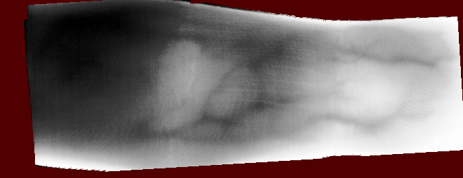
Fig. 1 Example RoI overlayed on finger vein image of the Vera fingervein database,
as produced by the script bob_bio_vein_view_sample.py.

Fig. 2 Example of fingervein image from the Vera fingervein database, binarized by using Maximum Curvature, after pre-processing.