Domain Specific Units
Many researchers pointed out that DCNNs progressively compute more powerful feature detectors as depth increases REF{Mallat2016}. The authors from REF{Yosinski2014} and REF{Hongyang2015} demonstrated that feature detectors that are closer to the input signal (called low level features) are base features that resemble Gabor features, color blobs, edge detectors, etc. On the other hand, features that are closer to the end of the neural network (called high level features) are considered to be more task specific and carry more discriminative power.
In first insights section we observed that the feature detectors from \(\mathcal{D}^s\) (VIS) have some discriminative power over all three target domains we have tested; with VIS-NIR being the “easiest” ones and the VIS-Thermal being the most challenging ones. With such experimental observations, we can draw the following hypothesis:
Note
Given \(X_s=\{x_1, x_2, ..., x_n\}\) and \(X_t=\{x_1, x_2, ..., x_n\}\) being a set of samples from \(\mathcal{D}^s\) and \(\mathcal{D}^t\), respectively, with their correspondent shared set of labels \(Y=\{y_1, y_2, ..., y_n\}\) and \(\Theta\) being all set of DCNN feature detectors from \(\mathcal{D}^s\) (already learnt), there are two consecutive subsets: one that is domain textbf{dependent}, \(\theta_t\), and one that is domain textbf{independent}, \(\theta_s\), where \(P(Y|X_s, \Theta) = P(Y|X_t, [\theta_s, \theta_t])\). Such \(\theta_t\), that can be learnt via back-propagation, is so called Domain Specific Units.
A possible assumption one can make is that \(\theta_t\) is part of the set of low level features, directly connected to the input signal. In this paper we test this assumption. Figure bellow presents a general schematic of our proposed approach. It is possible to observe that each image domain has its own specific set of feature detectors (low level features) and they share the same face space (high level features) that was previously learnt using VIS.
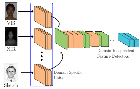
Our approach consists in learning \(\theta_t\), for each target domain, jointly with the DCNN from the source domain. In order to jointly learn \(\theta_t\) with \(D_s\) we propose two different architectural arrangements described in the next subsections.
Siamese DSU
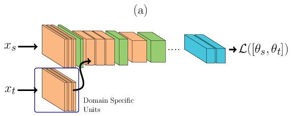
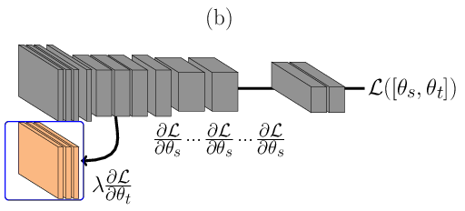
In the architecture described below, \(\theta_t\) is learnt using Siamese Neural Networks REF{Chopra2005}. During the forward pass, Figure (a), a pair of face images, one for each domain (either sharing the same identity or not), is passed through the DCNN. The image from the source domain is passed through the main network (the one at the top in Figure (a)) and the image from the target domain is passed first to its domain specific set of feature detectors and then amended to the main network. During the backward pass, Figure (b), errors are backpropagated only for \(\theta^t\). With such structure only a small subset of feature detectors are learnt, reducing the capacity of the joint model. The loss \(\mathcal{L}\) is defined as:
\(\mathcal{L}(\Theta) = 0.5\Bigg[ (1-Y)D(x_s, x_t) + Y \max(0, m - D(x_s, x_t))\Bigg]\), where \(m\) is the contrastive margin, \(Y\) is the label (1 when \(x_s\) and \(x_t\) belong to the same subject and 0 otherwise) and \(D\) is defined as:
\(D(x_s, x_t) = || \phi(x_s) - \phi(x_t)||_{2}^{2}\), where \(\phi\) are the embeddings from the jointly trained DCNN.
Results
Warning
Decribe the results from the paper
Understanding the Domain Specific Units
In this section we break down the covariate distribution of data points sensed in different image modalities layer by layer using tSNEs.
With these plots we expect to observe how data from different image modalities and different identities are organized along the DCNN transformations.
- For each image domain we present:
The covariate distribution using the base network as a reference (without any adaptation) in the left column.
The covariate distribution using the best DSU adapted network (for each database) in the right column.
For this analysis we make all the plots using the Inception Resnet v2 as a basis.
Pola Thermal
For this analysis, the columns on the right are generated using the \(\theta_{t[1-4]}\) DSU.
Pixel level distribution
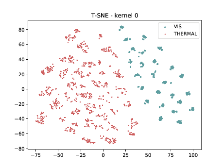
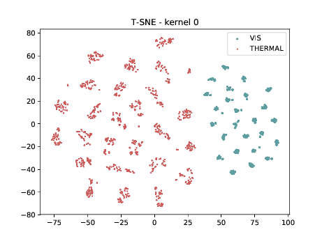
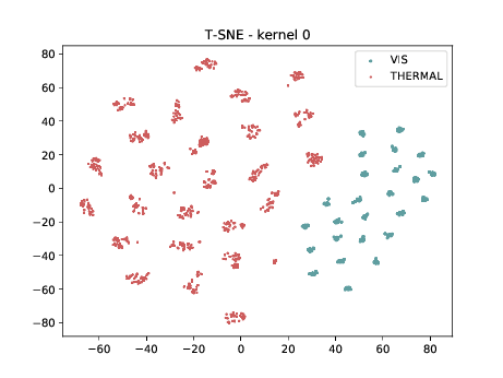
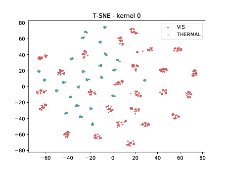
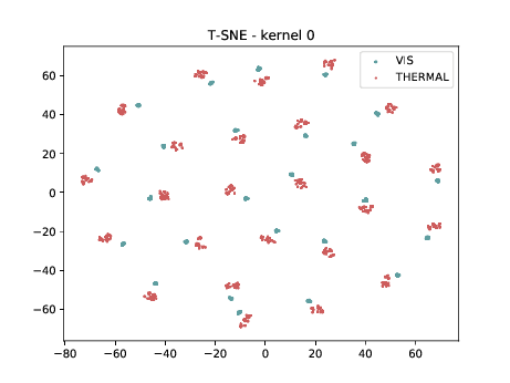
Below we present the tSNE covariate distribution using the pixels as input. Blue dots represent VIS samples and red dots represent Thermal samples. It’s possible to observe that images from different image modalities do cluster, which is an expected behaviour.
Conv2d_1a_3x3 (\(\theta_{t[1-1]}\) DSU adapted)
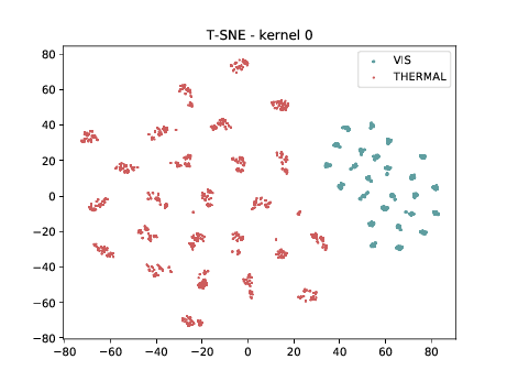
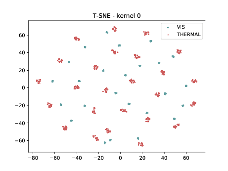
Below we present the tSNE covariate distribution using the output of the first layer as input (\(\theta_{1-1}\)). We can observe that in the very first layer the identities are clustered for both, adapted and non adapted, DCNNs. Moreover, the image modalities form two “big” clusters.
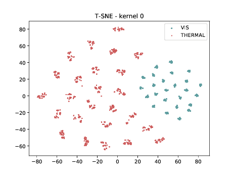
Conv2d_3b_1x1 (\(\theta_{t[1-2]}\) DSU adapted)
Below we present the tSNE covariate distribution using the output of the first layer as input (\(\theta_{1-2}\)). We can observe that in the very first layer the identities are clustered for both, adapted and non adapted, DCNNs. Moreover, the image modalities form two “big” clusters.
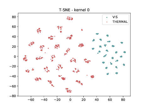
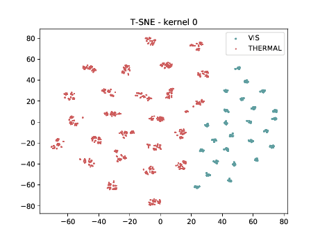
Conv2d_4a_3x3 (\(\theta_{t[1-4]}\) DSU adapted)
Below we present the tSNE covariate distribution using the output of the first layer as input (\(\theta_{1-4}\)). We can observe that in the very first layer the identities are clustered for both, adapted and non adapted, DCNNs. This is the last adapted layer for this setup and the image modalities are still organized in two different clusters, which is a behaviour that, at first glance, is not expected.
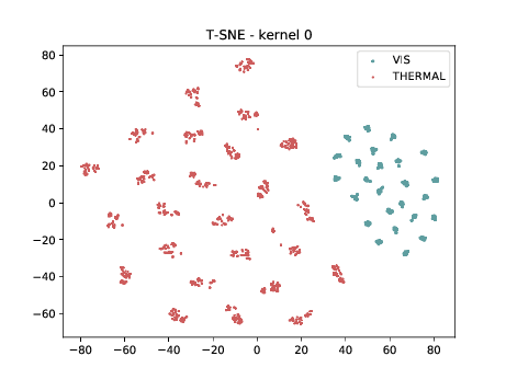
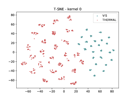
Mixed_5b (\(\theta_{t[1-5]}\))
From now, the layers are not DSU adapted. Below we can observe the same behaviour as before. Modalities are clustered in two “big” clusters and inside of these clusters, the identities are clustered.
Mixed_6a (\(\theta_{t[1-6]}\))
Below we can observe the same behaviour as before. Modalities are clustered in two “big” clusters and inside of these clusters, the identities are clustered.
Mixed_7a
Below we can observe the same behaviour as before. Modalities are clustered in two “big” clusters and inside of these clusters, the identities are clustered.
Conv2d_7b_1x1
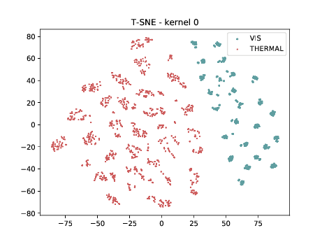
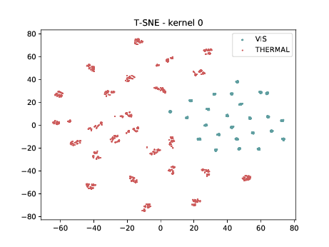
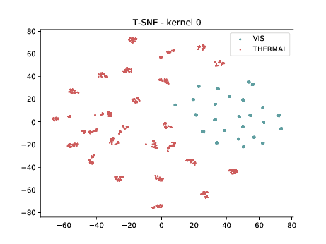
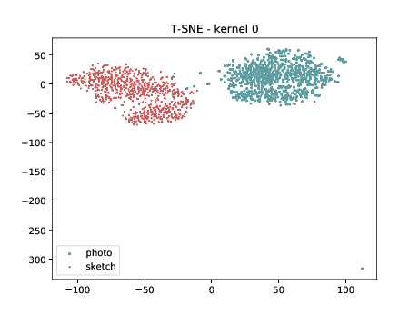
In the left tSNE (non DSU), we can observe the same behaviour as before. However, in the tSNE on the right we can observe that images from the same identities, but different image modalities start to cluster.
PreLogitsFlatten
In the left tSNE (non DSU), we can observe the same behaviour as before. However, in the tSNE on the right we can observe that images from the same identities, but different image modalities start to cluster. We can use this layer as the final embedding.
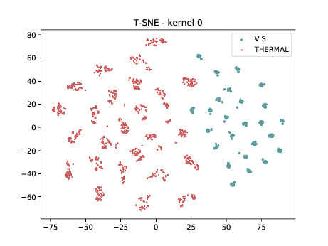
Final Embedding
In the left tSNE (non DSU), we can observe the same behaviour as before. However, in the tSNE on the right we can observe that images from the same identities, but different image modalities start to cluster. We can use this layer as the final embedding.
CUFSF
For this analysis, the columns on the right is generated using the \(\theta_{t[1-5]}\) DSU.
Pixel level distribution
Below we present the tSNE covariate distribution using the pixels as input. Blue dots represent VIS samples and red dots represents Thermal samples. It’s possible to observe that images from different image modalities do cluster, which is an expected behaviour.
Conv2d_1a_3x3 (\(\theta_{t[1-1]}\) DSU adapted)
Below we present the tSNE covariate distribution using the output of the first layer as input (\(\theta_{1-1}\)). We can observe that in the very first layer the identities are clustered (of course they are clustered, we have only one sample per identity/modality) for both, adapted and non adapted, DCNNs. Moreover, the image modalities form two “big” clusters.
Conv2d_3b_1x1 (\(\theta_{t[1-2]}\) DSU adapted)
Below we present the tSNE covariate distribution using the output of the first layer as input (\(\theta_{1-2}\)). We can observe that in the very first layer the identities are clustered (of course they are clustered, we have only one sample per identity/modality) for both, adapted and non adapted, DCNNs. Moreover, the image modalities form two “big” clusters.
Conv2d_4a_3x3 (\(\theta_{t[1-4]}\) DSU adapted)
Below we present the tSNE covariate distribution using the output of the first layer as input (\(\theta_{1-4}\)). We can observe that in the very first layer the identities are clustered (of course they are clustered, we have only one sample per identity/modality) for both, adapted and non adapted, DCNNs.
Mixed_5b (\(\theta_{t[1-5]}\) DSU adapted)
From now, the layers are not DSU adapted. Below we can observe the same behaviour as before. This is the last adapted layer for this setup and the image modalities are still organized in two different clusters, which is a behaviour that, at first glance, is not expected.
Mixed_6a (\(\theta_{t[1-6]}\))
Below we can observe the same behaviour as before. Modalities are clustered in two “big” clusters and inside of these clusters, the identities are clustered.
Mixed_7a
Below we can observe the same behaviour as before. Modalities are clustered in two “big” clusters and inside of these clusters, the identities are clustered.
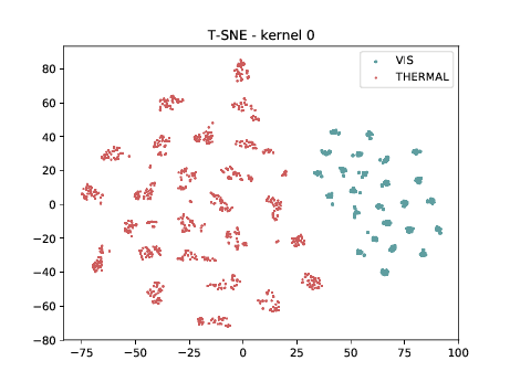
Conv2d_7b_1x1
In the left tSNE (non DSU), we can observe the same behaviour as before. However, in the tSNE on the right we can observe that images from the same identities, but different image modalities start to cluster.
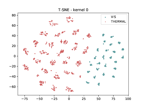
PreLogitsFlatten
In the left tSNE (non DSU), we can observe the same behaviour as before. However, in the tSNE on the right we can observe that images from the same identities, but different image modalities start to cluster. We can use this layer as the final embedding.
Final Embedding
In the left tSNE (non DSU), we can observe the same behaviour as before. However, in the tSNE on the right we can observe that images from the same identities, but different image modalities start to cluster. We can use this layer as the final embedding.
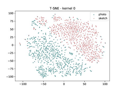
CUHK-CUFS
For this analysis, the columns on the right is generated using the \(\theta_{t[1-5]}\) DSU.
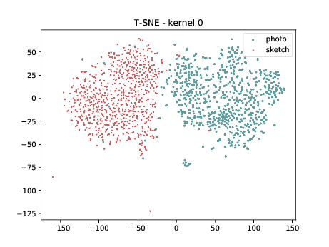
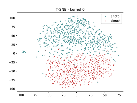
Pixel level distribution
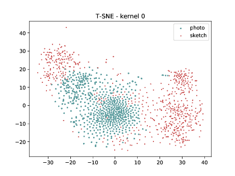
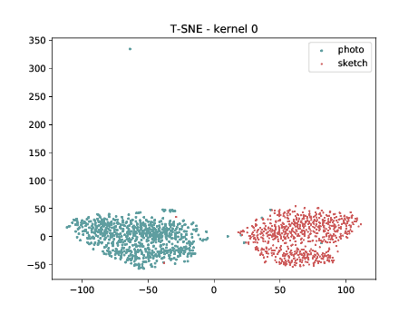
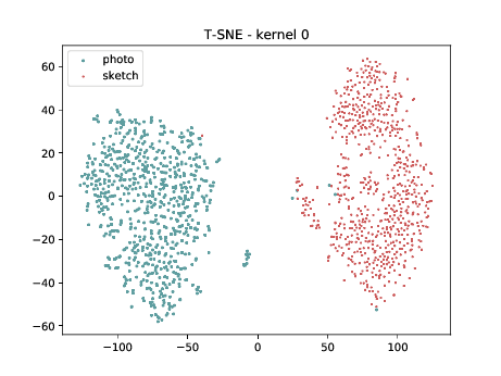
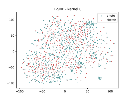
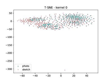
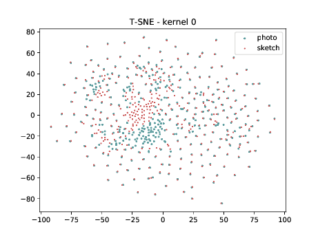
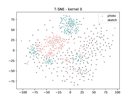
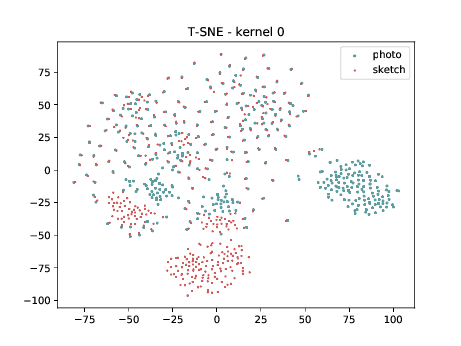
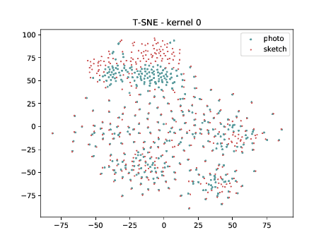
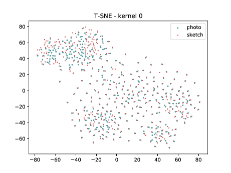
Below we present the tSNE covariate distribution using the pixels as input. Blue dots represent VIS samples and red dots represents Sketch samples. It’s possible to observe that images from different image modalities do cluster, which is an expected behaviour.
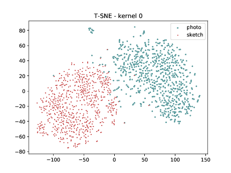
Conv2d_1a_3x3 (\(\theta_{t[1-1]}\) DSU adapted)
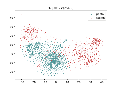
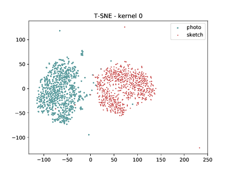
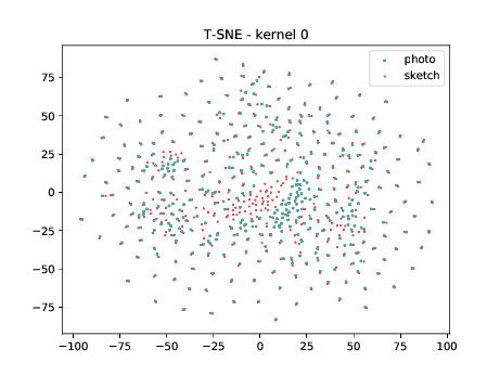
Below we present the tSNE covariate distribution using the output of the first layer as input (\(\theta_{1-1}\)). We can observe that from this layer, in both cases (left and right), images from different image modalities belongs to the same cluster. It’s not possible to use a linear classifier to classify both modalities. Moreover, the identities from different image modalities seems to form small clusters for some cases. For information, this database has only ONE pair of images sensed in both modalities.
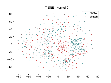
Conv2d_3b_1x1 (\(\theta_{t[1-2]}\) DSU adapted)
The same observation made in the last sub-section can be made for this case.
Conv2d_4a_3x3 (\(\theta_{t[1-4]}\) DSU adapted)
The same observation made in the last sub-section can be made for this case.
Mixed_5b (\(\theta_{t[1-5]}\) DSU adapted )
The same observation made in the last sub-section can be made for this case.
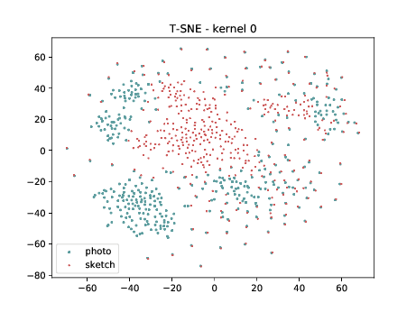
Mixed_6a (\(\theta_{t[1-6]}\))
The same observation made in the last sub-section can be made for this case.
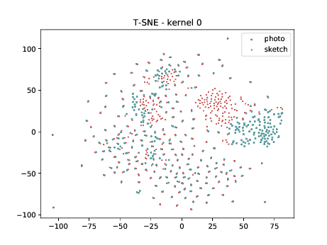
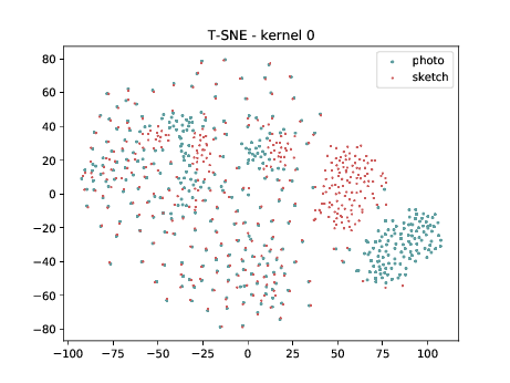
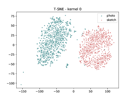
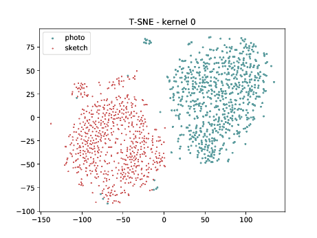
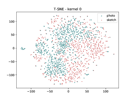
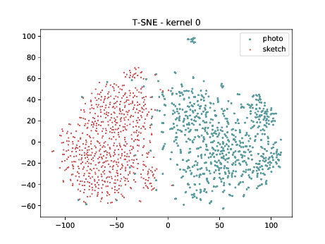
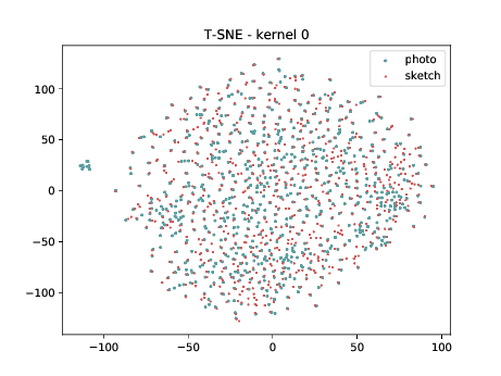
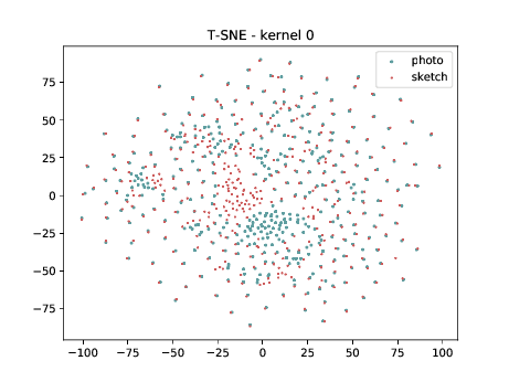
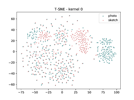
Conv2d_7b_1x1
The same observation made in the last sub-section can be made for this case. Overall, the same observation made in the last sub-section can be made for this case. We can observe some modality specific regions in the left plot, which can’t be observed in the plot on the right. Hence, it seems that the DSU has some effectiveness for this particular case.
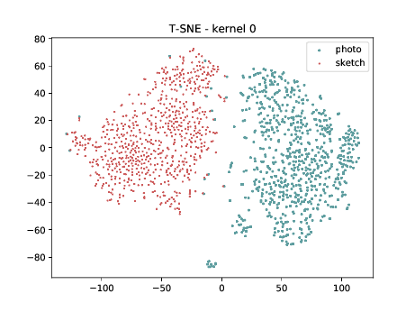
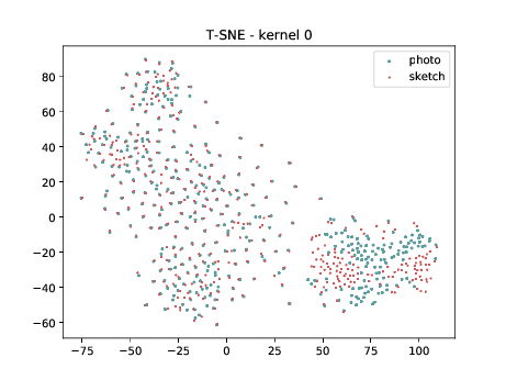
PreLogitsFlatten
The same observation made in the last sub-section can be made for this case. Overall, the same observation made in the last sub-section can be made for this case. We can observe some modality specific regions in the left plot, which can’t be observed in the plot on the right. Hence, it seems that the DSU has some effectiveness for this particular case.
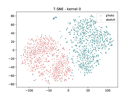
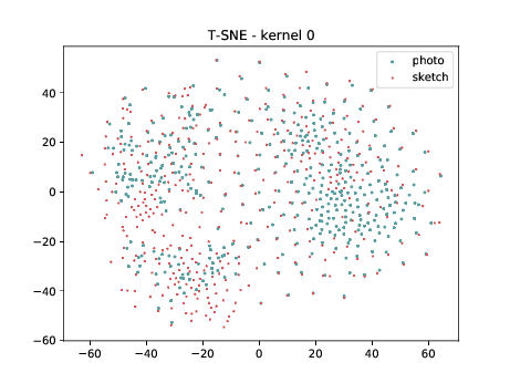
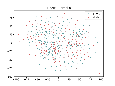
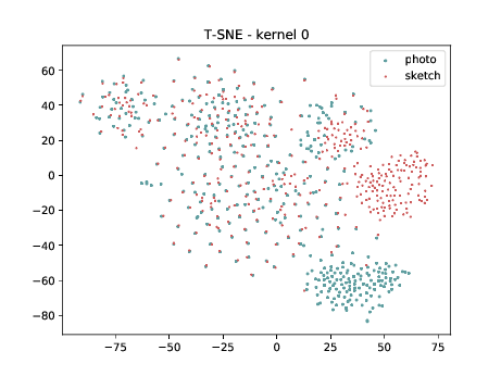
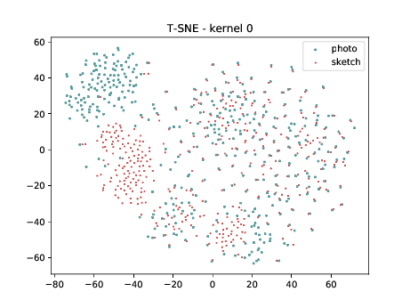
Final Embedding
Overall, the same observation made in the last sub-section can be made for this case. We can observe some modality specific regions in the left plot, which can’t be observed in the plot on the right. Hence, it seems that the DSU has some effectiveness for this particular case.
Triplet DSU
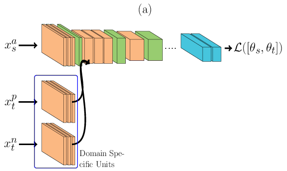
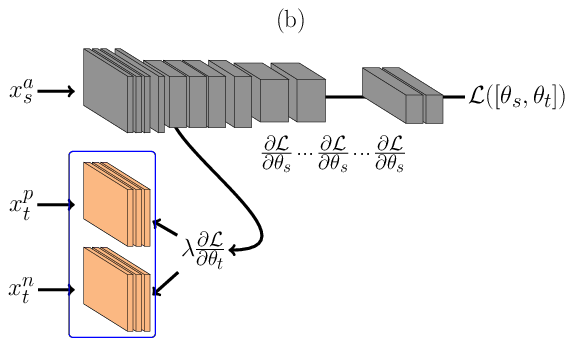
In the architecture described in Figure below, \(\theta_t\) is learnt using Triplet Neural Networks REF{Schroff2015}. During the forward pass, Figure (a), a triplet of face images are presented as inputs to the network. In its figure, \(x_s^{a}\) consist of face images sensed in the source domain, and \(x_t^{p}\) and \(x_t^{n}\) are images sensed in the target domain, where \(x_s^{a}\) and \(x_t^{p}\) are from the same identity and \(x_s^{a}\) and \(x_t^{n}\) are from different identities. As before, face images from the source domain are passed through the main network (the one at the top in Figure (a)) in and face images from the target domain are passed first to its domain specific set of feature detectors and then amended to the main network. During the backward pass, Figure (b), errors are backpropagated only for \(\theta^t\), that is shared between the inputs \(x_t^{p}\) and \(x_t^{n}\). With such structure only a small subset of features are learnt, reducing the capacity of the model. The loss \(\mathcal{L}\) is defined as:
\(\mathcal{L}(\theta) = ||\phi(x_s^{a}) - \phi(x_t^{p})||_2^{2} - ||\phi(x_s^{a}) - \phi(x_t^{n})||_2^{2} + \lambda\), where \(\lambda\) is the triplet margin and \(\phi\) are the embeddings from the DCNN.
For our experiments, two DCNN are chosen for \(D_s\): the Inception Resnet v1 and Inception Resnet v2. Such networks presented one of the highest recognition rates under different image domains. Since our target domains are one channel only, we selected the gray scaled version of it. Details of such architecture is presented in the Supplementary Material.
Our task is to find the set of low level feature detectors, \(\theta_t\), that maximizes the recognition rates for each image domain. In order to find such set, we exhaustively try, layer by layer (increasing the DCNN depth), adapting both Siamese and Triplet Networks. Five possible \(\theta_t\) sets are analysed and they are called \(\theta_{t[1-1]}\), \(\theta_{t[1-2]}\), \(\theta_{t[1-4]}\), \(\theta_{t[1-5]}\) and \(\theta_{t[1-6]}\). A full description of which layers compose \(\theta_t\) is presented in the Supplementary material of the paper. The Inception Resnet v2 architecture batch normalize REF[Ioffe2015] the forward signal for every layer. For convolutions, such batch normalization step is defined, for each layer \(i\), as the following:
\(h(x) = \beta_i + \frac{g{(W_i * x)} + \mu_i}{\sigma_i}\), where \(\beta\) is the batch normalization offset (role of the biases), \(W\) are the convolutional kernels, \(g\) is the non-linear function applied to the convolution (ReLU activation), \(\mu\) is the accumulated mean of the batch and \(\sigma\) is the accumulated standard deviation of the batch.
In the Equation, two variables are updated via backpropagation, the values of the kernel (\(W\)) and the offset (\(\beta\)). With these two variables, two possible scenarios for \(\theta_{t[1-n]}\) are defined. In the first scenario, we consider that \(\theta_{t[1-n]}\) is composed by the set of batch normalization offsets (\(\beta\)) only and the convolutional kernels \(W\) are shared between \(\mathcal{D}_s\) and \(\mathcal{D}_t\). We may hypothesize that, since the target object that we are trying to model has the same structure among domains (frontal faces with neutral expression most of the time), the feature detectors for \(\mathcal{D}_s\) and \(\mathcal{D}_t\), encoded in \(W\), are the same and just offsets need to be domain specific. In this work such models are represented as \(\theta_{t[1-n]}(\beta)\). In the second scenario, both \(W\) and \(\beta\) are made domain specific (updated via back-propagation) and they are represented as \(\theta_{t[1-n]}(\beta + W)\).