This page contains illustrations for video data:
Note that all results (also for synthetic data) have been obtained with the same concentration parameters (γ=2 and α=0.01), independently of the dataset.
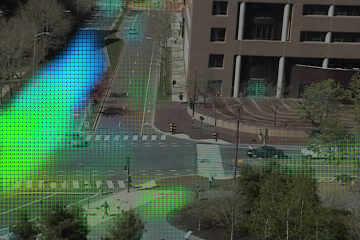
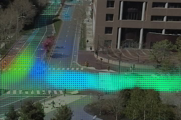
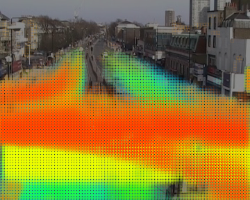
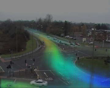
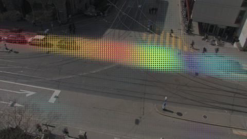
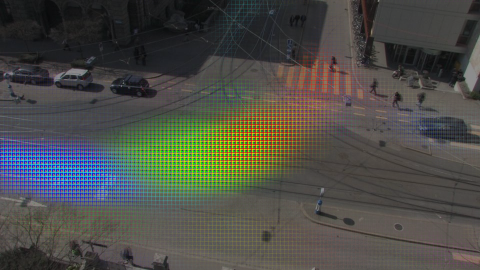
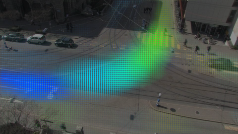
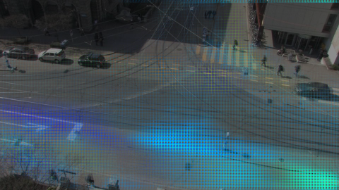
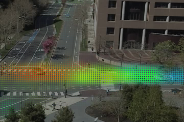
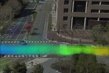
Given videos recorded from static cameras, we generate temporal documents by first applying a PLSA step on 1 second documents made of bag-of-words of low-level motion features. The posterior of these recovered topics at each time instant, weighted by the number of words, is used to build the input documents of our algorithm. Two sample documents are given below.
 |
| Temporal document for the “Far Field” video (300 seconds shown). This scene is not controlled by traffic lights so there are no particular cycles. |
  |
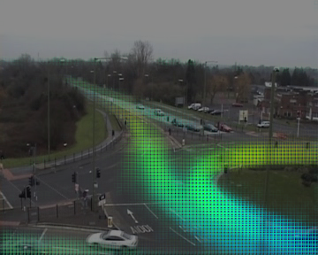
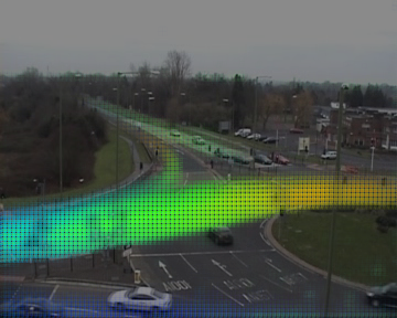
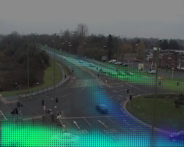
| Temporal document for the “MIT” video (300 seconds shown). This scene is controlled by traffic lights. We can observe some cycle of around 80 seconds. |
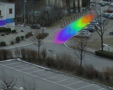
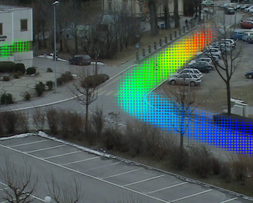
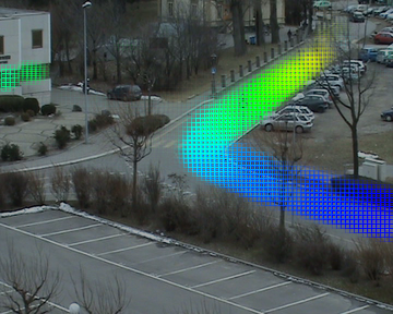
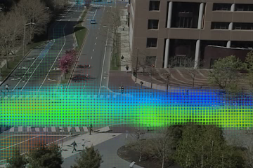
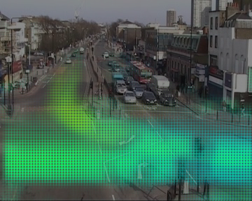
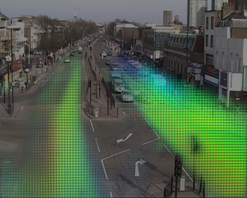
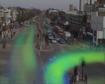
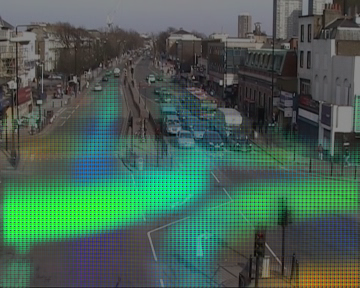
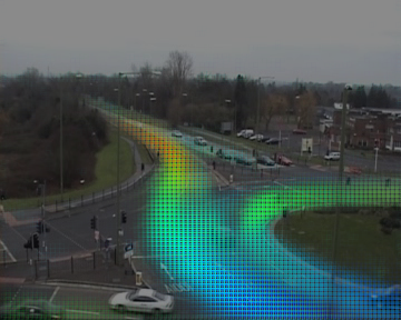
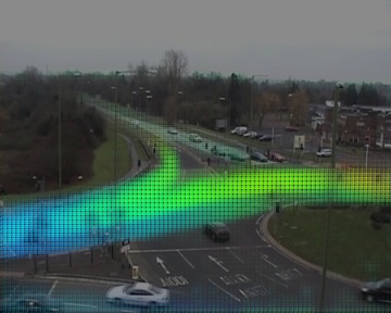
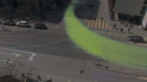
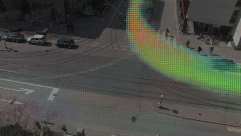
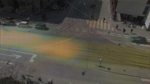
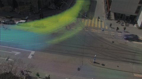
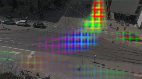
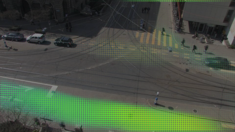
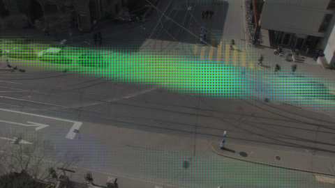
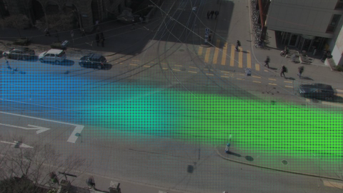
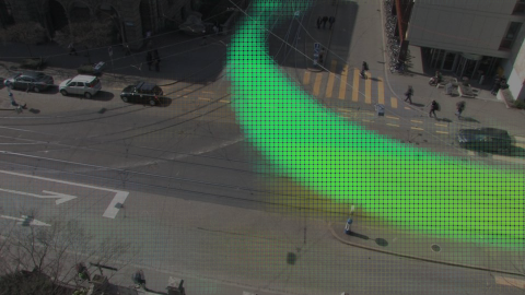
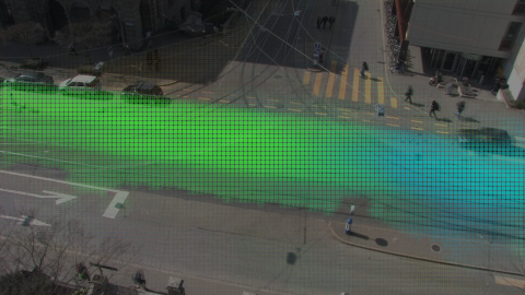
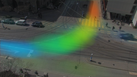
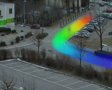
Each motif extracted using our algorithm can be interpreted as the probabilities of occurrence of each word at each relative time step. For video data, given the way our documents were constructed, we propose 3 different ways of representing the motifs (read from left to right):
 |
 |
 |
| (click image to replay) | ||
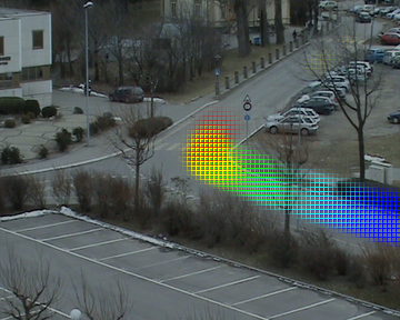
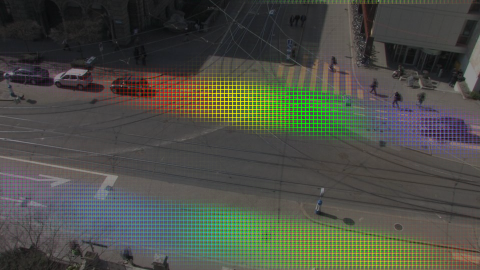
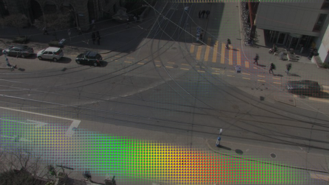
| This is the generic representation. The motif is displayed using a matrix image where white points represent a 0 probability and darker points represent higher probabilities. (you might spot the above motif in the first temporal document shown previously) | For video data, each word corresponds to a region of activity in the images. We can create a small animation by displaying in an image at each time step the backprojection of the words presents at that time step in the motif. By default, all animations are played at real speed. | We can create a static image by merging all time steps from the animation into a single image (as used in the article). |
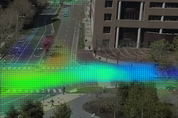
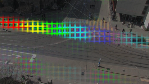
The color palette we use to represent evolution of time ranges from violet to red. The beginning of the motif is blue or violet (depending on whether the first time step is empty or not), the end is red. Red always represents the activity/words occurring at the maximal end of the motif, whatever the duration of the motif that was actually learned. Thus, if we seek for motifs of 20 seconds and that the learned topic is actually of length 10 seconds, we will not see red activities in the animation (and no intermediate green or orange either).
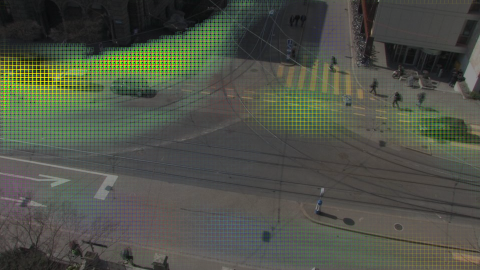
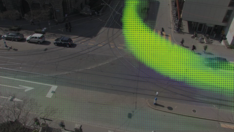
In our algorithm, we have to set the maximum duration for motifs to recover. We here show the impact of the “maximum motif duration” parameter of our model (comments after the images).
 |
 |
 |
| (max duration = 12 seconds) | (click image to replay) | |
| This first motif was recovered by our approach when seeking for motifs with a maximum duration of 12 seconds (12 time steps). We can notice that the actual activity is more or less of 12 seconds also. | ||
 |
 |
 |
| (max duration = 16 seconds) | (click image to replay) | |
|
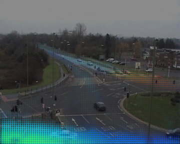
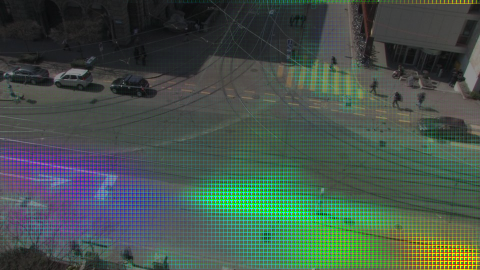
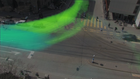
This second motif was learned when the maximum motif duration was set to 16 seconds.
Thanks to our use of a non-uniform prior on the motifs (Fig. 5 of the paper), the mass of the motif activity is located at the beginning of the the 16 seconds, leaving the end of the motif empty.
This phenomenon can be observed on all three representations: for example, no red is present on the colored representations, meaning that no words occur towards the end.
Notice that this example illustrate the robustness of our algorithm to motif duration setting: the same temporal pattern than in the first case is recovered even if a longer duration was sought. | ||
 |
 |
 |
| (click image to replay) | ||
|
|
|
| (max duration = 6 seconds) | (click image to replay) | |
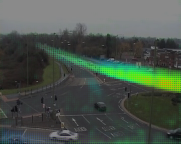
| When reducing the maximum duration of motifs to 6 seconds, we see that amongst the recovered motifs, two of them (the ones here) correspond to the 12 second motif shown at first. We notice that they are complementary: the second one most probably occurs after the first one. | ||
In the paper, we have shown visuals for the “far field” dataset with 11 second long motifs, and for MIT and UQM-Roundabout with 6 second long motifs. Here we show more results. We put a green border on images that we highlight in the comments below each set of images. We refer to motifs with their column and row number (e.g. c1r1 for the first motif, c1r2 for the fifth motif). Motifs ordered from the most probable to the less probable.
As we are using Gibbs sampling with Dirichlet Processes, the inference process is not strictly converging (Gibbs sampling generate state samples representing the true distribution). For interpretation purpose, we need to take a the state of the Gibbs sampler at a particular iteration. In the Gibbs sampling processes, new motifs can be created and destroyed. So the motifs present at a particular iteration might vary as shown in the graph below. To avoid showing newly created, low-importance motifs, we only show here the most probable motifs (as in Fig. 5 and Fig. 6 of the paper). Most of the time we remove between 1 and 5 motifs in the process.
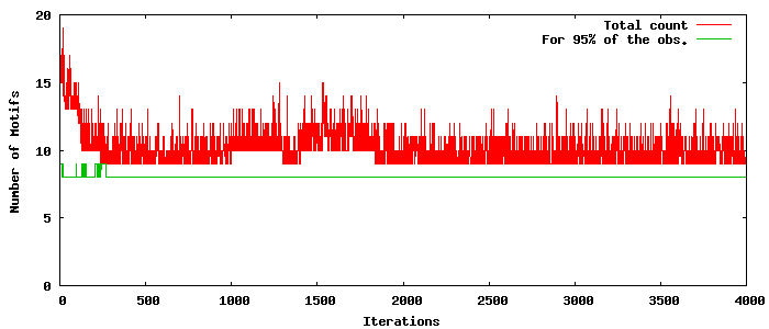 |
| Example of number of motifs through the iterations of the Gibbs sampler. |
 |
 |
 |
 |
 |
 |
 |
 |
Here again, we see that motifs are shorter than the maximum duration of 20 seconds as we see only little red. However, on this dataset, some “noise” (e.g. pedestrians) is captured by other unrelated motifs as in motif 7 (c3r2).
 |
 |
 |
 |
 |
 |
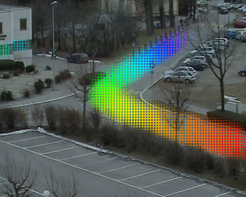
Please note that, in the UQM videos, cars are driving on the left side of the road. This dataset contains a lot of traffic, meaning a lot of co-occurring motion. The consequence is that the recovered motifs cover a bigger area at each time instant. We still recover the various phases of the traffic light cycle.
We capture important temporal information as in motif c2r2 where we see that i) (in blue) cars move up on the left of the image ii) then cars that were coming from the top and blocked by the moving up cars turn to their right and then iii) pedestrian crosses (yellow in the bottom right corner).
 |
 |
| (automatic loop, click to force restart) | |
| (accelerated ~4.5x) |
The scene is highly periodic with a period of almost 90 seconds. If we try to recover normal motifs (5 to 20 seconds) we do not capture the periodicity. As an experiment, we run our algorithm with 90 second long motifs. In the end, we obtain a single motif capturing the full cycle. We show it here as an animated gif (accelerated) as the static representation is here really obfuscated.
 |
 |
 |
 |
 |
 |
 |
 |
Here we observe the same phenomena as presented in the paper on Fig. 5: as there are important variations in execution speed of the activities, we recover multiple motifs looking almost the same (e.g. c2r1 and c4r1). The video is short (1 hour) so we also tend to capture fortuitous co-occurrences in the motifs (e.g. some light colored spots in c1r2).
 |
 |
 |
 |
 |
 |
 |
 |
 |
 |
 |
 |
 |
 |
On this dataset, we recover all the major car and tramway movements. We recover some interesting variation in trajectories. Observing c3r1 and c2r3, we see that they correspond to the same car lane but in c3r1 there is a brighter spot for cars before crossing the tramway rails. This activity corresponds to cars slowing down to wait for a tramway to finish crossing.
 |
 |
 |
 |
 |
 |
 |
 |
 |
 |
 |
Increasing the maximum duration of motifs to 16 seconds reveals that most of the activities are short (i.e. as captured in the case of 6 seconds in previous section). The only recovered motif that really spans the 16 seconds is c2r2, all other motifs having mostly no orange and red. We see also that c2r2 has a duplicate in c1r3 but with different execution speed: c1r3 corresponds to fast car turning while c2r2 is more for slower cars (e.g. because of pedestrians or tramway).
Tramways are big and cause long uniform motion patterns. That's why we hardly see the temporal information in c3r2. However, for faster cases of tramway, we get a slightly (c4r1) or really (c3r1) better temporal information.
Looking at the last motif (c3r3) we see that it captures both a tramway coming from the top to the left and a car waiting to cross from right to left. This event must be sufficiently recurrent to be captured in a motif.
Our method can be used for prediction, as shown in the paper.
 |
 |
||
 |
 |
 |
 |
| a) MIT dataset | b) Far field dataset | ||
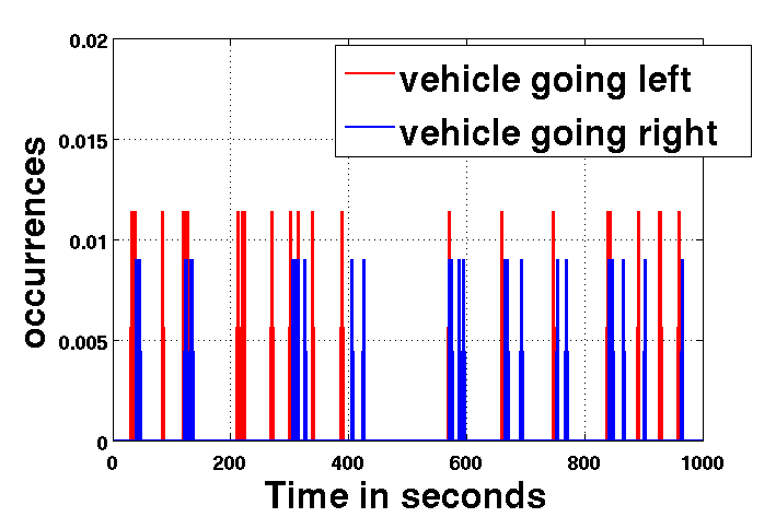
In the MIT data, activities are controlled by a traffic signal.
Due to the signal cycles, there are distinct global behavior patterns following
one-another in the scene.
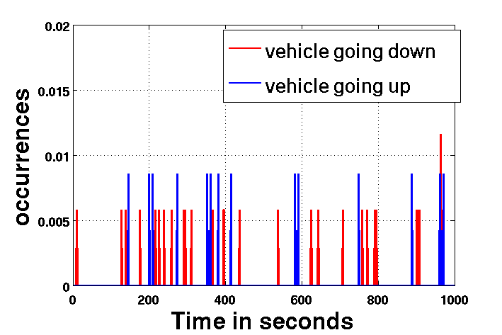
Occurrence plots of two activities automatically recovered by our algorithm
(vehicle moving left and vehicle moving right), are shown above.
From the curves, we can clearly see that these activities are
highly correlated temporally: blue activity is often occurring after a red one.
Such correlation can actually be observed for most of the activities in the scene.
Our method for activity prediction does not exploit such temporal dependencies
(although it could be extended to do so), to the contrary of the
Topic HMM we compare our algorithm to, which captures this recurring
pattern through its states and hence
provides a better prediction accuracy in this case.
In the second case, we see a similar plot of occurrences of two activities from the Farfield data( a)vehicle moving up and b) vehicle moving down). Here the scene is uncontrolled and hence no particular co-occurrence among activities can be observed as reflected in the plot. Therefore in such general cases, the Topic HMM method which specializes on global behavior sequence modeling does not perform better than our method which learns individual activities with strong temporal information.
