Multipie Dataset
Todo
Benchmarks on Multipie Database
Probably for Manuel’s students
Database
The CMU Multi-PIE face database contains more than 750,000 images of 337 people recorded in up to four sessions over the span of five months. Subjects were imaged under 15 view points and 19 illumination conditions while displaying a range of facial expressions. In addition, high resolution frontal images were acquired as well. In total, the database contains more than 305 GB of face data.
Content
The data has been recorded over 4 sessions. For each session, the subjects were asked to display a few different expressions. For each of those expressions, a complete set of 30 pictures is captured that includes 15 different view points times 20 different illumination conditions (18 with various flashes, plus 2 pictures with no flash at all).
Available expressions
Session 1 : neutral, smile
Session 2 : neutral, surprise, squint
Session 3 : neutral, smile, disgust
Session 4 : neutral, neutral, scream.
Camera and flash positioning
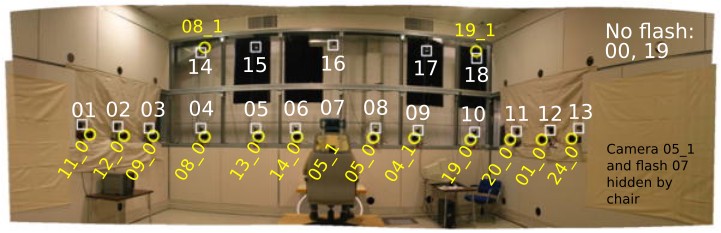
The different view points are obtained by a set of 13 cameras located at head height, spaced at 15° intervals, from the -90° to the 90° angle, plus 2 additional cameras located above the subject to simulate a typical surveillance view. A flash coincides with each camera, and 3 additional flashes are positioned above the subject, for a total of 18 different possible flashes.
The following picture showcase the positioning of the cameras (in yellow) and of the flashes (in white).
File paths
The data directory structure and filenames adopt the following structure:
session<XX>/multiview/<subject_id>/<recording_id>/<camera_id>/<subject_id>_<session_id>_<recording_id>_<camera_id>_<shot_id>.png
For example, the file
session02/multiview/001/02/05_1/001_02_02_051_07.png
corresponds to * Subject 001 * Session 2 * Second recording -> Expression is surprise * Camera 05_1 -> Frontal view * Shot 07 -> Illumination through the frontal flash
Protocols
Expression protocol
Protocol E
Only frontal view (camera 05_1); only no-flash (shot 0)
Enrolled : 1x neutral expression (session 1; recording 1)
Probes : 4x neutral expression + other expressions (session 2, 3, 4; all recordings)
Pose protocol
Protocol P
Only neutral expression (recording 1 from each session, + recording 2 from session 4); only no-flash (shot 0)
Enrolled : 1x frontal view (session 1; camera 05_1)
Probes : all views from cameras at head height (i.e excluding 08_1 and 19_1), including camera 05_1 from session 2,3,4.
Illumination protocols
N.B : shot 19 is never used in those protocols as it is redundant with shot 0 (both are no-flash).
Protocol M
Only frontal view (camera 05_1); only neutral expression (recording 1 from each session, + recording 2 from session 4)
Enrolled : no-flash (session 1; shot 0)
Probes : no-flash (session 2, 3, 4; shot 0)
Protocol U
Only frontal view (camera 05_1); only neutral expression (recording 1 from each session, + recording 2 from session 4)
Enrolled : no-flash (session 1; shot 0)
Probes : all shots from session 2, 3, 4, including shot 0.
Protocol G
Only frontal view (camera 05_1); only neutral expression (recording 1 from each session, + recording 2 from session 4)
Enrolled : all shots (session 1; all shots)
Probes : all shots from session 2, 3, 4.
Benchmarks
Run the baselines
You can run the Multipie baselines command with a simple command such as:
bob bio pipeline vanilla-biometrics multipie gabor_graph -m -l sge
Note that the default protocol implemented in the resource is the U protocol. The pose protocol is also available using
bob bio pipeline vanilla-biometrics multipie_pose gabor_graph -m -l sge
For the other protocols, one has to define its own configuration file (e.g.: multipie_M.py) as follows:
from bob.bio.face.database import MultipieDatabase
database = MultipieDatabase(protocol="M")
then point to it when calling the pipeline execution:
bob bio pipeline vanilla-biometrics multipie_M.py gabor_graph -m -l sge
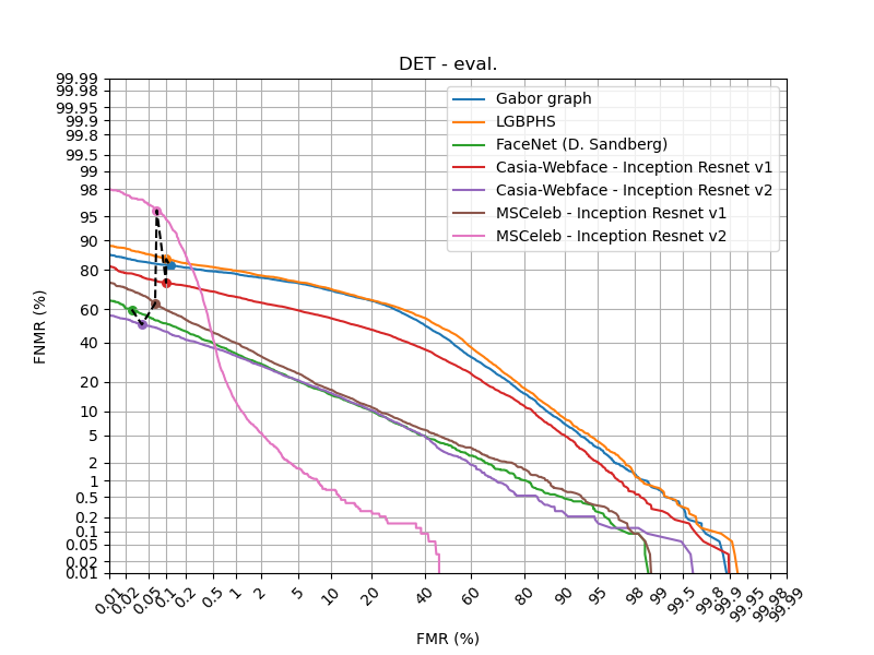
Leaderboard
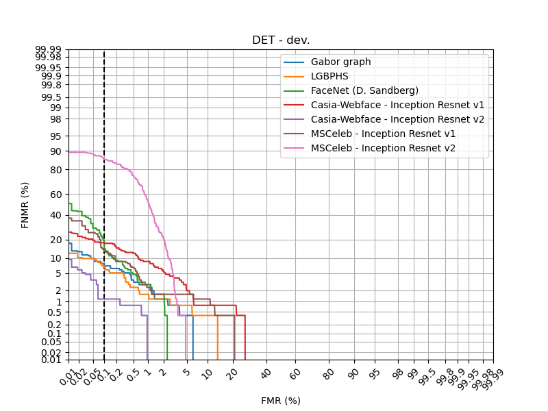
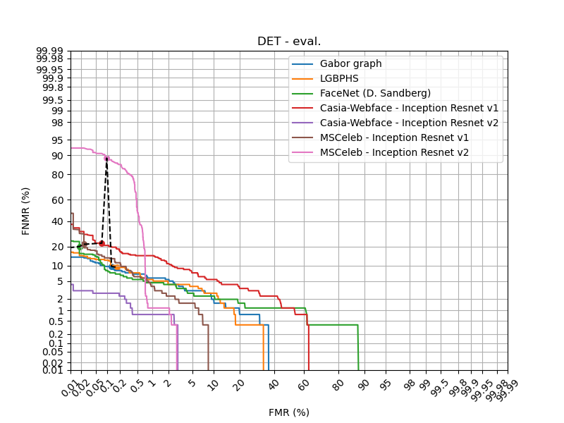
Protocol M
Baseline |
EER (dev) |
HTER (eval) |
|---|---|---|
Gabor graph |
1.26% |
3.68% |
LGBPHS |
1.17% |
3.06% |
FaceNet (D. Sandberg) |
1.56% |
2.74% |
Casia-Webface - Inception Resnet v1 |
3.83% |
5.98% |
Casia-Webface - Inception Resnet v2 |
0.76% |
0.74% |
MSCeleb - Inception Resnet v1 |
1.56% |
2.19% |
MSCeleb - Inception Resnet v2 |
3.09% |
7.09% |
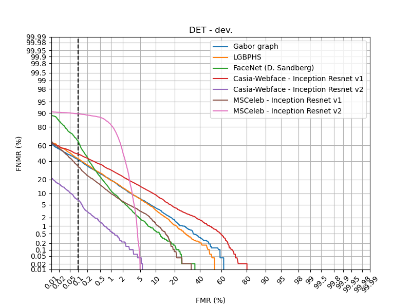
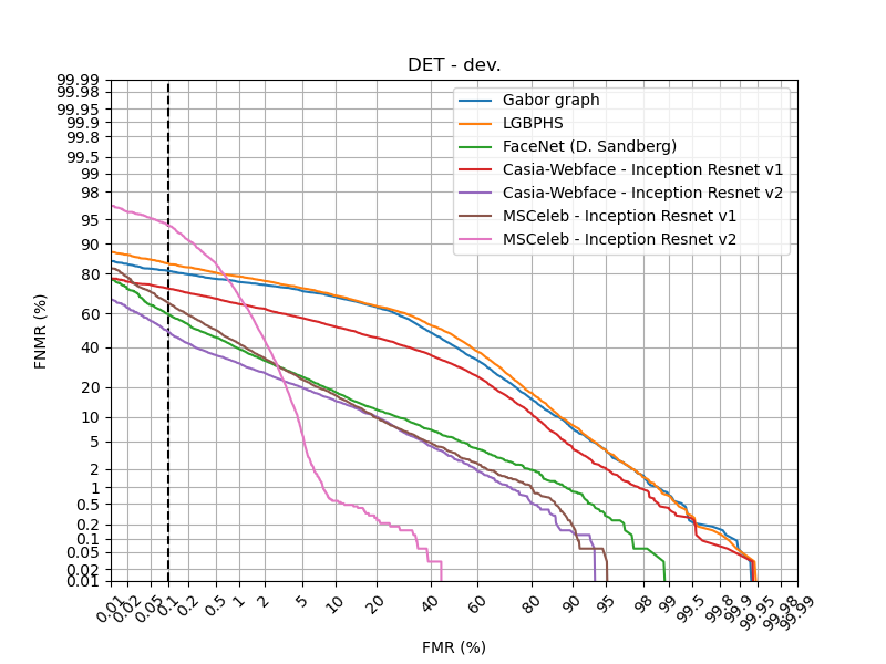
Protocol U
Baseline |
EER (dev) |
HTER (eval) |
|---|---|---|
Gabor graph |
6.25% |
7.44% |
LGBPHS |
6.02% |
6.85% |
FaceNet (D. Sandberg) |
3.31% |
3.56% |
Casia-Webface - Inception Resnet v1 |
9.50% |
9.43% |
Casia-Webface - Inception Resnet v2 |
0.80% |
1.46% |
MSCeleb - Inception Resnet v1 |
3.97% |
3.10% |
MSCeleb - Inception Resnet v2 |
3.82% |
6.54% |
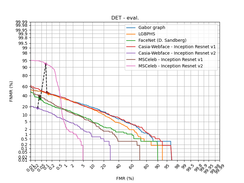
Protocol E
Baseline |
EER (dev) |
HTER (eval) |
|---|---|---|
Gabor graph |
14.24% |
15.56% |
LGBPHS |
13.36% |
13.78% |
FaceNet (D. Sandberg) |
5.21% |
6.64% |
Casia-Webface - Inception Resnet v1 |
12.89% |
13.67% |
Casia-Webface - Inception Resnet v2 |
2.11% |
3.07% |
MSCeleb - Inception Resnet v1 |
6.27% |
6.60% |
MSCeleb - Inception Resnet v2 |
3.82% |
4.46% |
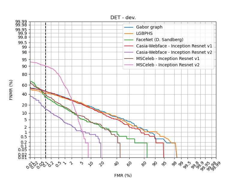
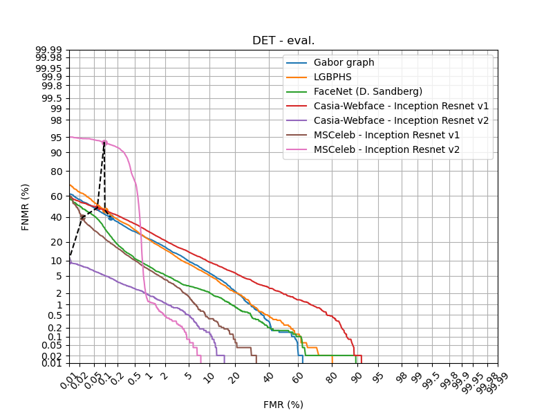
Protocol P
Baseline |
EER (dev) |
HTER (eval) |
|---|---|---|
Gabor graph |
44.83% |
45.66% |
LGBPHS |
48.23% |
48.36% |
FaceNet (D. Sandberg) |
14.46% |
13.93% |
Casia-Webface - Inception Resnet v1 |
37.23% |
37.11% |
Casia-Webface - Inception Resnet v2 |
13.04% |
13.12% |
MSCeleb - Inception Resnet v1 |
13.58% |
14.76% |
MSCeleb - Inception Resnet v2 |
5.17% |
5.22% |
For the pose protocol specifically, we can perform a more detailed study to assess angle-wise performance of the various FR systems. Hereafter is an example code to run this type of analysis, as well as the results. This code is also available as a Jupytext-compatible .py file under ./script/multipie/pose_analysis.py, that can be loaded as a Jupyter notebook.
import os
import pandas as pd
import bob.measure
import numpy as np
import matplotlib as mpl
mpl.rcParams.update({'font.size': 14})
import matplotlib.pyplot as plt
%matplotlib inline
Select baselines
baselines = {
    'Gabor graph': 'gabor_graph',
    'LGBPHS': 'lgbphs',
    'FaceNet (D. Sandberg)': 'facenet-sanderberg',
    'Casia-Webface - Inception Resnet v1': 'inception-resnetv1-casiawebface',
    'Casia-Webface - Inception Resnet v2': 'inception-resnetv2-casiawebface',
    'MSCeleb - Inception Resnet v1': 'inception-resnetv1-msceleb',
    'MSCeleb - Inception Resnet v2': 'inception-resnetv2-msceleb'
}
Define some utilitary functions
results_dir = './results/'

# Function to load the scores in CSV format
def load_scores(baseline, protocol, group):
    scores = pd.read_csv(os.path.join(results_dir,
                                      'multipie_{}'.format(protocol),
                                      baseline,
                                      'scores-{}.csv'.format(group)))
    return scores

# Function to separate genuines from impostors
def split(df):
    impostors = df[df['probe_reference_id'] != df['bio_ref_reference_id']]
    genuines = df[df['probe_reference_id'] == df['bio_ref_reference_id']]
    return impostors, genuines
Establish Camera to Angle conversion
cameras = ['11_0', '12_0','09_0','08_0','13_0','14_0','05_1','05_0', '04_1','19_0','20_0','01_0','24_0']
angles = np.linspace(-90, 90, len(cameras))
camera_to_angle = dict(zip(cameras, angles))
Run pose analysis and plot results
# Figure for Dev plot
fig1 = plt.figure(figsize=(8, 6))
# Figure for Eval plot
fig2 = plt.figure(figsize=(8, 6))
for name, baseline in baselines.items():

    # Load the score files and fill in the angle associated to each camera
    dev_scores = load_scores(baseline, 'P', 'dev')
    eval_scores = load_scores(baseline, 'P', 'eval')
    dev_scores['angle'] = dev_scores['probe_camera'].map(camera_to_angle)
    eval_scores['angle'] = eval_scores['probe_camera'].map(camera_to_angle)

    angles = []
    dev_hters = []
    eval_hters = []
    # Run the analysis per view angle
    for (angle, dev_df), (_, eval_df) in zip(dev_scores.groupby('angle'), eval_scores.groupby('angle')):
        # Separate impostors from genuines
        dev_impostors, dev_genuines = split(dev_df)
        eval_impostors, eval_genuines = split(eval_df)

        # Compute the min. HTER threshold on the Dev set
        threshold = bob.measure.min_hter_threshold(dev_impostors['score'], dev_genuines['score'])

        # Compute the HTER for the Dev and Eval set at this particular threshold
        dev_far, dev_frr = bob.measure.farfrr(dev_impostors['score'], dev_genuines['score'], threshold)
        eval_far, eval_frr = bob.measure.farfrr(eval_impostors['score'], eval_genuines['score'], threshold)
        angles.append(angle)
        dev_hters.append(1/2 * (dev_far + dev_frr))
        eval_hters.append(1/2 * (eval_far + eval_frr))

    # Update plots
    plt.figure(1)
    plt.plot(angles, dev_hters, label=name, marker='x')

    plt.figure(2)
    plt.plot(angles, eval_hters, label=name, marker='x')

# Plot finalization
plt.figure(1)
plt.title('Dev. min. HTER')
plt.xlabel('Angle')
plt.ylabel('Min HTER')
plt.legend()
plt.grid()

plt.figure(2)
plt.title('Eval. HTER @Dev min. HTER')
plt.xlabel('Angle')
plt.ylabel('HTER')
plt.legend()
plt.grid()

